Template fits
In applications we are interested in separating a signal component from background components, we often fit parameteric models to data. Sometimes constructing a parametric model for some component is difficult. In that case, one fits a template instead which may be obtained from simulation or from a calibration sample in which a pure component can be isolated.
The challenge then is to propagate the uncertainty of the template into the result. The template is now also estimated from a sample (be it simulated or a calibration sample), and the uncertainty associated to that can be substantial. We investigate different approaches for template fits, including the Barlow-Beeston and Barlow-Beeston-lite methods.
Note: This work has been published: H. Dembinski, A. Abdelmotteleb, Eur.Phys.J.C 82 (2022) 11, 1043
[1]:
from iminuit import Minuit
from iminuit.cost import poisson_chi2, Template, ExtendedBinnedNLL
import numpy as np
from scipy.stats import norm, truncexpon
from scipy.optimize import root_scalar, minimize
import matplotlib.pyplot as plt
from IPython.display import display
from collections import defaultdict
from joblib import Parallel, delayed
As a toy example, we generate a mixture of two components: a normally distributed signal and exponentially distributed background.
[2]:
def generate(rng, nmc, truth, bins):
    xe = np.linspace(0, 2, bins + 1)
    b = np.diff(truncexpon(1, 0, 2).cdf(xe))
    s = np.diff(norm(1, 0.1).cdf(xe))
    n = rng.poisson(b * truth[0]) + rng.poisson(s * truth[1])
    t = np.array([rng.poisson(b * nmc), rng.poisson(s * nmc)])
    return xe, n, t

rng = np.random.default_rng(1)
truth = 750, 250
xe, n, t = generate(rng, 100, truth, 15)
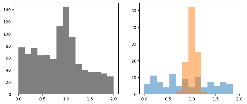
Data is visualized on the left-hand side. The templates are shown on the right-hand side. To show the effect of uncertainties in the template, this example intentially uses templates with poor statistical resolution.
[3]:
fig, ax = plt.subplots(1, 2, figsize=(10, 4), sharex=True)
ax[0].stairs(n, xe, fill=True, color="k", alpha=0.5, label="data")
for i, ti in enumerate(t):
    ax[1].stairs(ti, xe, fill=True, alpha=0.5, label=f"template {i}")
Bootstrapping template uncertainties
Bootstrapping is a general purpose technique to include uncertainties backed up by bootstrap theory, so it can be applied to this problem. We perform a standard fit and pretend that the templates have no uncertainties. Then, we repeat this fit many times with templates that are fluctuated around the actual values assuming a Poisson distribution.
Here is the cost function.
[4]:
def cost(yields):
    mu = 0
    for y, c in zip(yields, t):
        mu += y * c / np.sum(c)
    r = poisson_chi2(n, mu)
    return r

cost.errordef = Minuit.LEAST_SQUARES
cost.ndata = np.prod(n.shape)

starts = np.ones(2)
m = Minuit(cost, starts)
m.limits = (0, None)
m.migrad()
m.hesse()
[4]:
| Migrad | ||||
|---|---|---|---|---|
| FCN = 4.338e+04 (chi2/ndof = 3336.6) | Nfcn = 110 | |||
| EDM = 3.77e-06 (Goal: 0.0002) | ||||
| Valid Minimum | No Parameters at limit | |||
| Below EDM threshold (goal x 10) | Below call limit | |||
| Covariance | Hesse ok | Accurate | Pos. def. | Not forced |
| Name | Value | Hesse Error | Minos Error- | Minos Error+ | Limit- | Limit+ | Fixed | |
|---|---|---|---|---|---|---|---|---|
| 0 | x0 | 761 | 30 | 0 | ||||
| 1 | x1 | 193 | 19 | 0 |
| x0 | x1 | |
|---|---|---|
| x0 | 933 | -172 (-0.294) |
| x1 | -172 (-0.294) | 365 |
The uncertainties reported by the fit correspond to the uncertainty in the data, but not the uncertainty in the templates. The chi2/ndof is also very large, since the uncertainties in the template are not considered in the fit.
We bootstrap the templates 1000 times and compute the covariance of the fitted results.
[5]:
b = 100
rng = np.random.default_rng(1)
pars = []
for ib in range(b):
    ti = rng.poisson(t)

    def cost(yields):
        mu = 0
        for y, c in zip(yields, ti):
            mu += y * c / np.sum(c)
        r = poisson_chi2(n, mu)
        return r

    mi = Minuit(cost, m.values[:])
    mi.errordef = Minuit.LEAST_SQUARES
    mi.limits = (0, None)
    mi.strategy = 0
    mi.migrad()
    assert mi.valid
    pars.append(mi.values[:])

cov2 = np.cov(np.transpose(pars), ddof=1)
We print the uncertainties from the different stages and the correlation between the two yields.
To obtain the full error, we add the independent covariance matrices from the original fit and the bootstrap.
[6]:
cov1 = m.covariance

for title, cov in zip(("fit", "bootstrap", "fit+bootstrap"),
                      (cov1, cov2, cov1 + cov2)):
    print(title)
    for label, p, e in zip(("b", "s"), m.values, np.diag(cov) ** 0.5):
        print(f"  {label} {p:.0f} +- {e:.0f}")
    print(f"  correlation {cov[0, 1] / np.prod(np.diag(cov)) ** 0.5:.2f}")
fit
  b 761 +- 31
  s 193 +- 19
  correlation -0.29
bootstrap
  b 761 +- 36
  s 193 +- 36
  correlation -0.98
fit+bootstrap
  b 761 +- 47
  s 193 +- 40
  correlation -0.75
The bootstrapped template errors are much larger than the fit errors in this case, since the sample used to generate the templates is much smaller than the data sample.
The bootstrapped errors for both yields are nearly equal (they become exactly equal if the template sample is large) and the correlation is close to -1 (and becomes exactly -1 in large samples). This is expected, since the data sample is fixed in each iteration. Under these conditions, a change in the templates can only increase the yield of one component at an equal loss for the other component.
Template fit with nuisance parameters
As described in Barlow and Beeston, Comput.Phys.Commun. 77 (1993) 219-228, the correct treatment from first principles is to write down the likelihood function for this case, in which the observed values and unknown parameters are clearly stated. The insight is that the true contents of the bins for the templates are unknown and we need to introduce a nuisance parameter for each bin entry in the template. The combined likelihood for the problem is then combines the estimation of the template yields with the estimation of unknown templates.
This problem can be handled straight-forwardly with Minuit, but it leads to the introduction of a large number of nuisance parameters, one for each entry in each template. We again write a cost function for this case (here a class for convenience).
As a technical detail, it is necessary to increase the call limit in Migrad for the fit to fully converge, since the limit set by Minuit’s default heuristic is too tight for this application.
[7]:
class BB:
    def __init__(self, xe, n, t):
        self.xe = xe
        self.data = n, t

    def _pred(self, par):
        bins = len(self.xe) - 1
        yields = par[:2]
        nuisances = np.array(par[2:])
        b = nuisances[:bins]
        s = nuisances[bins:]
        mu = 0
        for y, c in zip(yields, (b, s)):
            mu += y * np.array(c) / np.sum(c)
        return mu, b, s

    def __call__(self, par):
        n, t = self.data
        mu, b, s = self._pred(par)
        r = poisson_chi2(n, mu) + poisson_chi2(t[0], b) + poisson_chi2(t[1], s)
        return r

    @property
    def ndata(self):
        n, t = self.data
        return np.prod(n.shape) + np.prod(t.shape)

    def visualize(self, args):
        n, t = self.data
        ne = n ** 0.5
        xe = self.xe
        cx = 0.5 * (xe[1:] + xe[:-1])
        plt.errorbar(cx, n, ne, fmt="ok")
        mu = 0
        mu_var = 0
        for y, c in zip(args[:2], t):
            f = 1 / np.sum(c)
            mu += c * y * f
            mu_var += c * (f * y) ** 2
        mu_err = mu_var ** 0.5
        plt.stairs(mu + mu_err, xe, baseline=mu - mu_err, fill=True, color="C0")
        # plt.stairs(mu, xe, color="C0")

m1 = Minuit(BB(xe, n, t), np.concatenate([truth, t[0], t[1]]))
m1.limits = (0, None)
m1.migrad(ncall=100000)
m1.hesse()
[7]:
| Migrad | ||||
|---|---|---|---|---|
| FCN = 18.27 (chi2/ndof = 1.4) | Nfcn = 3464 | |||
| EDM = 6.02e-05 (Goal: 0.0002) | ||||
| Valid Minimum | SOME Parameters at limit | |||
| Below EDM threshold (goal x 10) | Below call limit | |||
| Covariance | Hesse ok | Accurate | Pos. def. | Not forced |
| Name | Value | Hesse Error | Minos Error- | Minos Error+ | Limit- | Limit+ | Fixed | |
|---|---|---|---|---|---|---|---|---|
| 0 | x0 | 800 | 50 | 0 | ||||
| 1 | x1 | 190 | 40 | 0 | ||||
| 2 | x2 | 9.0 | 1.4 | 0 | ||||
| 3 | x3 | 8.5 | 1.3 | 0 | ||||
| 4 | x4 | 9.0 | 1.4 | 0 | ||||
| 5 | x5 | 7.4 | 1.2 | 0 | ||||
| 6 | x6 | 8.4 | 1.3 | 0 | ||||
| 7 | x7 | 6.4 | 1.1 | 0 | ||||
| 8 | x8 | 9.2 | 1.7 | 0 | ||||
| 9 | x9 | 4.8 | 2.3 | 0 | ||||
| 10 | x10 | 7.0 | 1.5 | 0 | ||||
| 11 | x11 | 5.5 | 1.0 | 0 | ||||
| 12 | x12 | 5.1 | 0.9 | 0 | ||||
| 13 | x13 | 4.6 | 0.9 | 0 | ||||
| 14 | x14 | 4.7 | 0.9 | 0 | ||||
| 15 | x15 | 4.3 | 0.8 | 0 | ||||
| 16 | x16 | 3.2 | 0.7 | 0 | ||||
| 17 | x17 | 0.0 | 0.4 | 0 | ||||
| 18 | x18 | 0.0 | 0.4 | 0 | ||||
| 19 | x19 | 0.0 | 0.4 | 0 | ||||
| 20 | x20 | 0.0 | 0.5 | 0 | ||||
| 21 | x21 | 0.0 | 0.4 | 0 | ||||
| 22 | x22 | 2.1 | 1.5 | 0 | ||||
| 23 | x23 | 19 | 4 | 0 | ||||
| 24 | x24 | 54 | 7 | 0 | ||||
| 25 | x25 | 23 | 4 | 0 | ||||
| 26 | x26 | 1.1 | 1.0 | 0 | ||||
| 27 | x27 | 0.0 | 0.4 | 0 | ||||
| 28 | x28 | 0.0 | 0.4 | 0 | ||||
| 29 | x29 | 0.0 | 0.4 | 0 | ||||
| 30 | x30 | 0.0 | 0.4 | 0 | ||||
| 31 | x31 | 0.0 | 0.5 | 0 |
| x0 | x1 | x2 | x3 | x4 | x5 | x6 | x7 | x8 | x9 | x10 | x11 | x12 | x13 | x14 | x15 | x16 | x17 | x18 | x19 | x20 | x21 | x22 | x23 | x24 | x25 | x26 | x27 | x28 | x29 | x30 | x31 | |
|---|---|---|---|---|---|---|---|---|---|---|---|---|---|---|---|---|---|---|---|---|---|---|---|---|---|---|---|---|---|---|---|---|
| x0 | 2.24e+03 | -1.45e+03 (-0.756) | -14.6 (-0.226) | -13.8 (-0.222) | -14.6 (-0.226) | -12 (-0.214) | -13.6 (-0.221) | -5.25 (-0.100) | 23.6 (0.289) | 68.9 (0.644) | 23.2 (0.320) | -6.29 (-0.134) | -8.3 (-0.191) | -7.42 (-0.184) | -7.59 (-0.185) | -7.06 (-0.181) | -5.12 (-0.161) | 2.82e-08 | -0 | -1.04e-06 | -2.67e-06 | -0 | -5.71 (-0.081) | -26.2 (-0.131) | 29.8 (0.089) | 5.32 (0.026) | -3.16 (-0.062) | -0 | -0 | -0 | -0 | -2.52e-05 |
| x1 | -1.45e+03 (-0.756) | 1.64e+03 | 14.6 (0.264) | 13.8 (0.260) | 14.6 (0.264) | 12 (0.250) | 13.6 (0.259) | 5.25 (0.117) | -23.6 (-0.338) | -68.9 (-0.754) | -23.2 (-0.375) | 6.29 (0.157) | 8.3 (0.223) | 7.42 (0.215) | 7.59 (0.217) | 7.06 (0.212) | 5.12 (0.188) | -2.72e-08 | 0 | 1.03e-06 | 2.66e-06 | 0 | 5.71 (0.095) | 26.2 (0.153) | -29.8 (-0.104) | -5.32 (-0.030) | 3.16 (0.073) | 0 | 0 | 0 | 0 | 2.52e-05 |
| x2 | -14.6 (-0.226) | 14.6 (0.264) | 1.88 | 0.842 (0.470) | 0.895 (0.477) | 0.734 (0.452) | 0.831 (0.468) | 0.584 (0.384) | 0.525 (0.222) | -0.302 (-0.098) | 0.345 (0.165) | 0.522 (0.384) | 0.507 (0.403) | 0.453 (0.389) | 0.464 (0.392) | 0.432 (0.382) | 0.313 (0.340) | 2.37e-09 | 0 | 9.87e-09 | 2.43e-08 | 0 | 0.0578 (0.028) | 0.264 (0.046) | -0.3 (-0.031) | -0.0538 (-0.009) | 0.0319 (0.022) | 0 | 0 | 0 | 0 | 2.62e-07 |
| x3 | -13.8 (-0.222) | 13.8 (0.260) | 0.842 (0.470) | 1.71 | 0.842 (0.470) | 0.69 (0.445) | 0.781 (0.460) | 0.549 (0.378) | 0.494 (0.218) | -0.284 (-0.096) | 0.324 (0.162) | 0.491 (0.378) | 0.477 (0.397) | 0.426 (0.382) | 0.436 (0.385) | 0.406 (0.376) | 0.294 (0.334) | -1.08e-10 | -0 | 8.99e-09 | 2.28e-08 | 0 | 0.0543 (0.028) | 0.248 (0.045) | -0.282 (-0.031) | -0.0505 (-0.009) | 0.03 (0.021) | 0 | 0 | 0 | 0 | 2.48e-07 |
| x4 | -14.6 (-0.226) | 14.6 (0.264) | 0.895 (0.477) | 0.842 (0.470) | 1.88 | 0.734 (0.452) | 0.831 (0.468) | 0.584 (0.384) | 0.525 (0.222) | -0.302 (-0.098) | 0.345 (0.165) | 0.522 (0.384) | 0.507 (0.403) | 0.453 (0.389) | 0.464 (0.392) | 0.432 (0.382) | 0.313 (0.340) | -1.07e-10 | 0 | -7.03e-08 | 2.45e-08 | 0 | 0.0578 (0.028) | 0.264 (0.046) | -0.3 (-0.031) | -0.0537 (-0.009) | 0.0319 (0.022) | 0 | 0 | 0 | 0 | 2.62e-07 |
| x5 | -12 (-0.214) | 12 (0.250) | 0.734 (0.452) | 0.69 (0.445) | 0.734 (0.452) | 1.4 | 0.681 (0.443) | 0.478 (0.364) | 0.431 (0.210) | -0.248 (-0.092) | 0.283 (0.156) | 0.428 (0.364) | 0.416 (0.382) | 0.372 (0.368) | 0.38 (0.371) | 0.354 (0.362) | 0.256 (0.322) | -9.87e-11 | 0 | 7.25e-09 | -1.65e-07 | 0 | 0.0473 (0.027) | 0.216 (0.043) | -0.246 (-0.029) | -0.0441 (-0.009) | 0.0262 (0.021) | 0 | 0 | 0 | 0 | 2.16e-07 |
| x6 | -13.6 (-0.221) | 13.6 (0.259) | 0.831 (0.468) | 0.781 (0.460) | 0.831 (0.468) | 0.681 (0.443) | 1.68 | 0.541 (0.376) | 0.487 (0.218) | -0.28 (-0.096) | 0.32 (0.162) | 0.484 (0.377) | 0.471 (0.396) | 0.421 (0.381) | 0.431 (0.384) | 0.401 (0.375) | 0.29 (0.333) | -1.17e-10 | 0 | 8.8e-09 | 2.29e-08 | -0 | 0.0536 (0.028) | 0.245 (0.045) | -0.278 (-0.030) | -0.0499 (-0.009) | 0.0296 (0.021) | 0 | 0 | 0 | 0 | 2.43e-07 |
| x7 | -5.25 (-0.100) | 5.25 (0.117) | 0.584 (0.384) | 0.549 (0.378) | 0.584 (0.384) | 0.478 (0.364) | 0.541 (0.376) | 1.23 | 0.421 (0.220) | -0.0401 (-0.016) | 0.295 (0.174) | 0.346 (0.314) | 0.331 (0.325) | 0.295 (0.313) | 0.302 (0.315) | 0.281 (0.307) | 0.204 (0.273) | -1.31e-11 | 0 | 5.87e-09 | 1.39e-08 | 0 | -0.424 (-0.258) | 0.207 (0.044) | 0.116 (0.015) | 0.0813 (0.017) | 0.0193 (0.016) | 0 | 0 | 0 | 0 | 1.4e-07 |
| x8 | 23.6 (0.289) | -23.6 (-0.338) | 0.525 (0.222) | 0.494 (0.218) | 0.525 (0.222) | 0.431 (0.210) | 0.487 (0.218) | 0.421 (0.220) | 2.99 | 0.999 (0.256) | 0.732 (0.277) | 0.348 (0.203) | 0.298 (0.188) | 0.266 (0.181) | 0.272 (0.182) | 0.253 (0.178) | 0.184 (0.158) | 4.8e-11 | 0 | 1.44e-09 | -1.43e-09 | 0 | 0.0195 (0.008) | -3.03 (-0.416) | 2.16 (0.177) | 0.842 (0.112) | 0.00754 (0.004) | 0 | 0 | 0 | 0 | -7.48e-08 |
| x9 | 68.9 (0.644) | -68.9 (-0.754) | -0.302 (-0.098) | -0.284 (-0.096) | -0.302 (-0.098) | -0.248 (-0.092) | -0.28 (-0.096) | -0.0401 (-0.016) | 0.999 (0.256) | 5.1 | 0.934 (0.271) | -0.0941 (-0.042) | -0.171 (-0.083) | -0.153 (-0.079) | -0.157 (-0.080) | -0.146 (-0.078) | -0.106 (-0.070) | 1.73e-10 | 0 | -1.09e-08 | -3.64e-08 | 0 | -0.048 (-0.014) | 0.432 (0.045) | -2.1 (-0.132) | 1.75 (0.178) | -0.0329 (-0.014) | 0 | 0 | 0 | 0 | -5.36e-07 |
| x10 | 23.2 (0.320) | -23.2 (-0.375) | 0.345 (0.165) | 0.324 (0.162) | 0.345 (0.165) | 0.283 (0.156) | 0.32 (0.162) | 0.295 (0.174) | 0.732 (0.277) | 0.934 (0.271) | 2.33 | 0.238 (0.157) | 0.195 (0.139) | 0.175 (0.134) | 0.179 (0.135) | 0.166 (0.132) | 0.12 (0.117) | 1.13e-12 | 0 | 4.71e-11 | -4.1e-09 | 0 | 0.00938 (0.004) | 0.336 (0.052) | 1.97 (0.183) | -2.32 (-0.349) | 0.0023 | 0 | 0 | 0 | 0 | -1.01e-07 |
| x11 | -6.29 (-0.134) | 6.29 (0.157) | 0.522 (0.384) | 0.491 (0.378) | 0.522 (0.384) | 0.428 (0.364) | 0.484 (0.377) | 0.346 (0.314) | 0.348 (0.203) | -0.0941 (-0.042) | 0.238 (0.157) | 0.984 | 0.296 (0.325) | 0.264 (0.313) | 0.271 (0.315) | 0.252 (0.307) | 0.182 (0.273) | -9.79e-11 | 0 | 5.47e-09 | 1.33e-08 | 0 | 0.0327 (0.022) | 0.172 (0.041) | -0.0118 (-0.002) | 0.0295 (0.007) | -0.223 (-0.211) | 0 | 0 | 0 | 0 | 1.37e-07 |
| x12 | -8.3 (-0.191) | 8.3 (0.223) | 0.507 (0.403) | 0.477 (0.397) | 0.507 (0.403) | 0.416 (0.382) | 0.471 (0.396) | 0.331 (0.325) | 0.298 (0.188) | -0.171 (-0.083) | 0.195 (0.139) | 0.296 (0.325) | 0.843 | 0.257 (0.328) | 0.263 (0.331) | 0.245 (0.323) | 0.177 (0.287) | -7.11e-11 | 0 | 4.86e-09 | 1.39e-08 | 0 | 0.0327 (0.024) | 0.149 (0.039) | -0.17 (-0.026) | -0.0305 (-0.008) | 0.0181 | -0 | 0 | 0 | 0 | 1.5e-07 |
| x13 | -7.42 (-0.184) | 7.42 (0.215) | 0.453 (0.389) | 0.426 (0.382) | 0.453 (0.389) | 0.372 (0.368) | 0.421 (0.381) | 0.295 (0.313) | 0.266 (0.181) | -0.153 (-0.079) | 0.175 (0.134) | 0.264 (0.313) | 0.257 (0.328) | 0.726 | 0.235 (0.319) | 0.219 (0.311) | 0.158 (0.277) | -6.73e-11 | 0 | 4.78e-09 | 1.24e-08 | 0 | 0.0292 (0.023) | 0.133 (0.037) | -0.152 (-0.025) | -0.0272 (-0.007) | 0.0162 (0.018) | 0 | -0 | 0 | 0 | 1.34e-07 |
| x14 | -7.59 (-0.185) | 7.59 (0.217) | 0.464 (0.392) | 0.436 (0.385) | 0.464 (0.392) | 0.38 (0.371) | 0.431 (0.384) | 0.302 (0.315) | 0.272 (0.182) | -0.157 (-0.080) | 0.179 (0.135) | 0.271 (0.315) | 0.263 (0.331) | 0.235 (0.319) | 0.749 | 0.224 (0.313) | 0.162 (0.279) | -5.43e-11 | 0 | 4.48e-09 | 1.29e-08 | 0 | 0.0299 (0.023) | 0.137 (0.037) | -0.155 (-0.025) | -0.0279 (-0.007) | 0.0165 (0.018) | 0 | 0 | -0 | 0 | 1.37e-07 |
| x15 | -7.06 (-0.181) | 7.06 (0.212) | 0.432 (0.382) | 0.406 (0.376) | 0.432 (0.382) | 0.354 (0.362) | 0.401 (0.375) | 0.281 (0.307) | 0.253 (0.178) | -0.146 (-0.078) | 0.166 (0.132) | 0.252 (0.307) | 0.245 (0.323) | 0.219 (0.311) | 0.224 (0.313) | 0.681 | 0.151 (0.272) | -5.74e-11 | 0 | 4.48e-09 | 1.21e-08 | 0 | 0.0278 (0.023) | 0.127 (0.037) | -0.145 (-0.025) | -0.0259 (-0.007) | 0.0154 (0.017) | 0 | 0 | 0 | -0 | 1.27e-07 |
| x16 | -5.12 (-0.161) | 5.12 (0.188) | 0.313 (0.340) | 0.294 (0.334) | 0.313 (0.340) | 0.256 (0.322) | 0.29 (0.333) | 0.204 (0.273) | 0.184 (0.158) | -0.106 (-0.070) | 0.12 (0.117) | 0.182 (0.273) | 0.177 (0.287) | 0.158 (0.277) | 0.162 (0.279) | 0.151 (0.272) | 0.452 | -7.57e-11 | 0 | 3.32e-09 | 9.14e-09 | 0 | 0.0202 | 0.0921 (0.033) | -0.105 (-0.022) | -0.0188 (-0.006) | 0.0111 (0.016) | 0 | 0 | 0 | 0 | -1.25e-06 |
| x17 | 2.82e-08 | -2.72e-08 | 2.37e-09 | -1.08e-10 | -1.07e-10 | -9.87e-11 | -1.17e-10 | -1.31e-11 | 4.8e-11 | 1.73e-10 | 1.13e-12 | -9.79e-11 | -7.11e-11 | -6.73e-11 | -5.43e-11 | -5.74e-11 | -7.57e-11 | 4.96e-09 | 0 | -1.06e-15 | 4.24e-14 | -0 | -6.61e-11 | 3.35e-10 | 8.66e-10 | 4.04e-10 | 6.92e-12 | 0 | 0 | -0 | -0 | -1.87e-13 |
| x18 | -0 | 0 | 0 | -0 | 0 | 0 | 0 | 0 | 0 | 0 | 0 | 0 | 0 | 0 | 0 | 0 | 0 | 0 | 0 | 0 | -0 | -0 | 0 | 0 | 0 | 0 | 0 | -0 | -0 | 0 | -0 | 0 |
| x19 | -1.04e-06 | 1.03e-06 | 9.87e-09 | 8.99e-09 | -7.03e-08 | 7.25e-09 | 8.8e-09 | 5.87e-09 | 1.44e-09 | -1.09e-08 | 4.71e-11 | 5.47e-09 | 4.86e-09 | 4.78e-09 | 4.48e-09 | 4.48e-09 | 3.32e-09 | -1.06e-15 | 0 | 5.45e-07 | -1.29e-13 | 0 | 6.39e-10 | 2.48e-09 | -1.99e-08 | -6.18e-09 | -2.06e-10 | 0 | 0 | 0 | 0 | -8.77e-13 |
| x20 | -2.67e-06 | 2.66e-06 | 2.43e-08 | 2.28e-08 | 2.45e-08 | -1.65e-07 | 2.29e-08 | 1.39e-08 | -1.43e-09 | -3.64e-08 | -4.1e-09 | 1.33e-08 | 1.39e-08 | 1.24e-08 | 1.29e-08 | 1.21e-08 | 9.14e-09 | 4.24e-14 | -0 | -1.29e-13 | 6.59e-07 | -0 | 1.99e-09 | 5.74e-10 | -7.53e-08 | -2.41e-08 | 1.21e-09 | -0 | -0 | -0 | -0 | 6.71e-13 |
| x21 | -0 | 0 | 0 | 0 | 0 | 0 | -0 | 0 | 0 | 0 | 0 | 0 | 0 | 0 | 0 | 0 | 0 | -0 | -0 | 0 | -0 | 0 | 0 | 0 | 0 | 0 | 0 | -0 | -0 | -0 | -0 | 0 |
| x22 | -5.71 (-0.081) | 5.71 (0.095) | 0.0578 (0.028) | 0.0543 (0.028) | 0.0578 (0.028) | 0.0473 (0.027) | 0.0536 (0.028) | -0.424 (-0.258) | 0.0195 (0.008) | -0.048 (-0.014) | 0.00938 (0.004) | 0.0327 (0.022) | 0.0327 (0.024) | 0.0292 (0.023) | 0.0299 (0.023) | 0.0278 (0.023) | 0.0202 | -6.61e-11 | 0 | 6.39e-10 | 1.99e-09 | 0 | 2.19 | 0.0106 (0.002) | -0.0762 (-0.007) | -0.0247 (-0.004) | 0.00233 | 0 | 0 | 0 | 0 | 2.55e-08 |
| x23 | -26.2 (-0.131) | 26.2 (0.153) | 0.264 (0.046) | 0.248 (0.045) | 0.264 (0.046) | 0.216 (0.043) | 0.245 (0.045) | 0.207 (0.044) | -3.03 (-0.416) | 0.432 (0.045) | 0.336 (0.052) | 0.172 (0.041) | 0.149 (0.039) | 0.133 (0.037) | 0.137 (0.037) | 0.127 (0.037) | 0.0921 (0.033) | 3.35e-10 | 0 | 2.48e-09 | 5.74e-10 | 0 | 0.0106 (0.002) | 17.8 | 0.947 (0.032) | 0.371 (0.020) | 0.00444 (0.001) | 0 | 0 | 0 | 0 | -1.79e-08 |
| x24 | 29.8 (0.089) | -29.8 (-0.104) | -0.3 (-0.031) | -0.282 (-0.031) | -0.3 (-0.031) | -0.246 (-0.029) | -0.278 (-0.030) | 0.116 (0.015) | 2.16 (0.177) | -2.1 (-0.132) | 1.97 (0.183) | -0.0118 (-0.002) | -0.17 (-0.026) | -0.152 (-0.025) | -0.155 (-0.025) | -0.145 (-0.025) | -0.105 (-0.022) | 8.66e-10 | 0 | -1.99e-08 | -7.53e-08 | 0 | -0.0762 (-0.007) | 0.947 (0.032) | 49.8 | 3.46 (0.113) | -0.0548 (-0.007) | 0 | 0 | 0 | 0 | -9.96e-07 |
| x25 | 5.32 (0.026) | -5.32 (-0.030) | -0.0538 (-0.009) | -0.0505 (-0.009) | -0.0537 (-0.009) | -0.0441 (-0.009) | -0.0499 (-0.009) | 0.0813 (0.017) | 0.842 (0.112) | 1.75 (0.178) | -2.32 (-0.349) | 0.0295 (0.007) | -0.0305 (-0.008) | -0.0272 (-0.007) | -0.0279 (-0.007) | -0.0259 (-0.007) | -0.0188 (-0.006) | 4.04e-10 | 0 | -6.18e-09 | -2.41e-08 | 0 | -0.0247 (-0.004) | 0.371 (0.020) | 3.46 (0.113) | 18.9 | -0.0184 (-0.004) | 0 | 0 | 0 | 0 | -3.5e-07 |
| x26 | -3.16 (-0.062) | 3.16 (0.073) | 0.0319 (0.022) | 0.03 (0.021) | 0.0319 (0.022) | 0.0262 (0.021) | 0.0296 (0.021) | 0.0193 (0.016) | 0.00754 (0.004) | -0.0329 (-0.014) | 0.0023 | -0.223 (-0.211) | 0.0181 | 0.0162 (0.018) | 0.0165 (0.018) | 0.0154 (0.017) | 0.0111 (0.016) | 6.92e-12 | 0 | -2.06e-10 | 1.21e-09 | 0 | 0.00233 | 0.00444 (0.001) | -0.0548 (-0.007) | -0.0184 (-0.004) | 1.14 | 0 | 0 | 0 | 0 | 1.54e-08 |
| x27 | -0 | 0 | 0 | 0 | 0 | 0 | 0 | 0 | 0 | 0 | 0 | 0 | -0 | 0 | 0 | 0 | 0 | 0 | -0 | 0 | -0 | -0 | 0 | 0 | 0 | 0 | 0 | 0 | -0 | -0 | -0 | 0 |
| x28 | -0 | 0 | 0 | 0 | 0 | 0 | 0 | 0 | 0 | 0 | 0 | 0 | 0 | -0 | 0 | 0 | 0 | 0 | -0 | 0 | -0 | -0 | 0 | 0 | 0 | 0 | 0 | -0 | 0 | -0 | -0 | 0 |
| x29 | -0 | 0 | 0 | 0 | 0 | 0 | 0 | 0 | 0 | 0 | 0 | 0 | 0 | 0 | -0 | 0 | 0 | -0 | 0 | 0 | -0 | -0 | 0 | 0 | 0 | 0 | 0 | -0 | -0 | 0 | -0 | 0 |
| x30 | -0 | 0 | 0 | 0 | 0 | 0 | 0 | 0 | 0 | 0 | 0 | 0 | 0 | 0 | 0 | -0 | 0 | -0 | -0 | 0 | -0 | -0 | 0 | 0 | 0 | 0 | 0 | -0 | -0 | -0 | 0 | 0 |
| x31 | -2.52e-05 | 2.52e-05 | 2.62e-07 | 2.48e-07 | 2.62e-07 | 2.16e-07 | 2.43e-07 | 1.4e-07 | -7.48e-08 | -5.36e-07 | -1.01e-07 | 1.37e-07 | 1.5e-07 | 1.34e-07 | 1.37e-07 | 1.27e-07 | -1.25e-06 | -1.87e-13 | 0 | -8.77e-13 | 6.71e-13 | 0 | 2.55e-08 | -1.79e-08 | -9.96e-07 | -3.5e-07 | 1.54e-08 | 0 | 0 | 0 | 0 | 5.19e-06 |
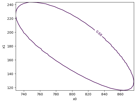
The result of this fit is comparable to the bootstrap method for this example, but the chi2/ndof is now reasonable and the uncertainties are correct without further work. This method should perform better than the bootstrap method, if the count per bin in the templates is small.
Another advantage is of this technique is that one can profile over the likelihood to obtain a 2D confidence regions, which is not possible with the bootstrap technique.
[8]:
m1.draw_mncontour("x0", "x1");
Before moving on, we briefly explore a possible refinement of the previous method, which is to hide the nuisance parameters from Minuit with a nested fit. It turns out that this technique is not an improvement, but it is useful to show that explicitly.
The idea is to construct an outer cost function, which only has the yields as parameters. Inside the outer cost function, the best nuisance parameters are found for the current yields with an inner cost function. Technically, this is achieved by calling a minimizer on the inner cost function at every call to the outer cost function.
Technical detail: It is important here to adjust Minuit’s expectation of how accurate the cost function is computed. Usually, Minuit performs its internal calculations under the assumption that the cost function is accurate to machine precision. This is usually not the case when a minimizer is used internally to optimize the inner function. We perform the internal minimization with SciPy, which allows us to set the tolerance. We set it here to 1e-8, which is sufficient for this problem and saves a bit of time on the internal minimisation. We then instruct Minuit to expect only this precision.
[9]:
precision = 1e-8

def cost(yields):
    bins = len(n)

    def inner(nuisance):
        b = nuisance[:bins]
        s = nuisance[bins:]
        mu = 0
        for y, c in zip(yields, (b, s)):
            mu += y * c / np.sum(c)
        r = poisson_chi2(n, mu) + poisson_chi2(t[0], b) + poisson_chi2(t[1], s)
        return r

    bounds = np.zeros((2 * bins, 2))
    bounds[:, 1] = np.inf
    r = minimize(inner, np.ravel(t), bounds=bounds, tol=precision)
    assert r.success
    return r.fun

cost.errordef = Minuit.LEAST_SQUARES
cost.ndata = np.prod(n.shape)

m2 = Minuit(cost, truth)
m2.precision = precision
m2.limits = (0, None)
m2.migrad()
m2.hesse()
[9]:
| Migrad | ||||
|---|---|---|---|---|
| FCN = 18.27 (chi2/ndof = 1.4) | Nfcn = 60 | |||
| EDM = 2.94e-08 (Goal: 0.0002) | ||||
| Valid Minimum | No Parameters at limit | |||
| Below EDM threshold (goal x 10) | Below call limit | |||
| Covariance | Hesse ok | Accurate | Pos. def. | Not forced |
| Name | Value | Hesse Error | Minos Error- | Minos Error+ | Limit- | Limit+ | Fixed | |
|---|---|---|---|---|---|---|---|---|
| 0 | x0 | 800 | 50 | 0 | ||||
| 1 | x1 | 190 | 40 | 0 |
| x0 | x1 | |
|---|---|---|
| x0 | 2.24e+03 | -1.45e+03 (-0.756) |
| x1 | -1.45e+03 (-0.756) | 1.64e+03 |
We obtain the exact same result as expected, but the runtime is much longer (more than a factor 10), which disfavors this technique compared to the straight-forward fit. The minimization is not as efficient, because Minuit cannot exploit correlations between the internal and the external parameters that allow it to converge it faster when it sees all parameters at once.
Template fits
The implementation described by Barlow and Beeston, Comput.Phys.Commun. 77 (1993) 219-228 solves the problem similarly to the nested fit described above, but the solution to the inner problem is found with an efficient algorithm.
The Barlow-Beeston approach still requires numerically solving a non-linear equation per bin. Several authors tried to replace the stop with approximations. - Conway, PHYSTAT 2011, https://arxiv.org/abs/1103.0354 uses an approximation in which the optimal nuisance parameters can be found by bin-by-bin by solving a quadratic equation which has only one allowed solution. - C.A. Argüelles, A. Schneider, T. Yuan, JHEP 06 (2019) 030 use a Bayesian treatment in which the uncertainty from the finite size of the simulation sample is modeled with a prior (which is itself a posterior conditioned on the simulation result). A closed formula for the likelihood can be derived. - H. Dembinski, A. Abdelmotteleb, Eur.Phys.J.C 82 (2022) 11, 1043 derived an approximation similar to Conway, but which treats data and simulation symmetrically.
All three methods are implemented in the built-in Template cost function (see documentation for details).
[10]:
c = Template(n, xe, t, method="jsc") # Conway
m3 = Minuit(c, *truth)
m3.limits = (0, None)
m3.migrad()
m3.hesse()
[10]:
| Migrad | ||||
|---|---|---|---|---|
| FCN = 11.52 (chi2/ndof = 0.9) | Nfcn = 48 | |||
| EDM = 6.05e-05 (Goal: 0.0002) | ||||
| Valid Minimum | No Parameters at limit | |||
| Below EDM threshold (goal x 10) | Below call limit | |||
| Covariance | Hesse ok | Accurate | Pos. def. | Not forced |
| Name | Value | Hesse Error | Minos Error- | Minos Error+ | Limit- | Limit+ | Fixed | |
|---|---|---|---|---|---|---|---|---|
| 0 | x0 | 0.86e3 | 0.11e3 | 0 | ||||
| 1 | x1 | 190 | 40 | 0 |
| x0 | x1 | |
|---|---|---|
| x0 | 1.16e+04 | -1.56e+03 (-0.330) |
| x1 | -1.56e+03 (-0.330) | 1.94e+03 |
[11]:
c = Template(n, xe, t, method="asy") # Argüelles, Schneider, Yuan
m4 = Minuit(c, *truth)
m4.limits = (0, None)
m4.migrad()
m4.hesse()
[11]:
| Migrad | ||||
|---|---|---|---|---|
| FCN = 61.24 | Nfcn = 43 | |||
| EDM = 1.03e-05 (Goal: 0.0001) | ||||
| Valid Minimum | No Parameters at limit | |||
| Below EDM threshold (goal x 10) | Below call limit | |||
| Covariance | Hesse ok | Accurate | Pos. def. | Not forced |
| Name | Value | Hesse Error | Minos Error- | Minos Error+ | Limit- | Limit+ | Fixed | |
|---|---|---|---|---|---|---|---|---|
| 0 | x0 | 660 | 70 | 0 | ||||
| 1 | x1 | 210 | 40 | 0 |
| x0 | x1 | |
|---|---|---|
| x0 | 5.25e+03 | -838 (-0.290) |
| x1 | -838 (-0.290) | 1.59e+03 |
[12]:
c = Template(n, xe, t, method="da") # Dembinski, Abdelmotteleb
m5 = Minuit(c, *truth)
m5.limits = (0, None)
m5.migrad()
m5.hesse()
[12]:
| Migrad | ||||
|---|---|---|---|---|
| FCN = 11.42 (chi2/ndof = 0.9) | Nfcn = 47 | |||
| EDM = 1.85e-06 (Goal: 0.0002) | ||||
| Valid Minimum | No Parameters at limit | |||
| Below EDM threshold (goal x 10) | Below call limit | |||
| Covariance | Hesse ok | Accurate | Pos. def. | Not forced |
| Name | Value | Hesse Error | Minos Error- | Minos Error+ | Limit- | Limit+ | Fixed | |
|---|---|---|---|---|---|---|---|---|
| 0 | x0 | 760 | 90 | 0 | ||||
| 1 | x1 | 190 | 40 | 0 |
| x0 | x1 | |
|---|---|---|
| x0 | 8.08e+03 | -1.26e+03 (-0.329) |
| x1 | -1.26e+03 (-0.329) | 1.81e+03 |
[13]:
for title, m in zip(("full fit", "T(JSC)", "T(ASY)", "T(DA)"), (m1, m3, m4, m5)):
    print(title)
    cov = m.covariance
    for label, p, e in zip(("x0", "x1"), m.values, np.diag(cov) ** 0.5):
        print(f"  {label} {p:.0f} +- {e:.0f}")
    print(f"  correlation {cov[0, 1] / (cov[0, 0] * cov[1, 1]) ** 0.5:.2f}")
full fit
  x0 796 +- 47
  x1 187 +- 40
  correlation -0.76
T(JSC)
  x0 858 +- 108
  x1 185 +- 44
  correlation -0.33
T(ASY)
  x0 660 +- 72
  x1 205 +- 40
  correlation -0.29
T(DA)
  x0 762 +- 90
  x1 194 +- 43
  correlation -0.33
The yields found by the approximate Template methods (T) differ from those found with the exact Barlow-Beeston likelihood (BB) method, because the likelihoods are different. In this particular case, the uncertainty for the signal estimated by the Template methods is larger, but this not the case in general.
The difference shows up in particular in the 68 % confidence regions.
[14]:
c1 = m1.mncontour("x0", "x1")
c3 = m3.mncontour("x0", "x1")
c4 = m4.mncontour("x0", "x1")
c5 = m5.mncontour("x0", "x1")
plt.plot(c1[:,0], c1[:, 1], label="BB")
plt.plot(c3[:,0], c3[:, 1], label="T(JSC)")
plt.plot(c4[:,0], c4[:, 1], label="T(ASY)")
plt.plot(c5[:,0], c4[:, 1], label="T(DA)")
plt.xlabel("background yield")
plt.ylabel("signal yield")
plt.legend();
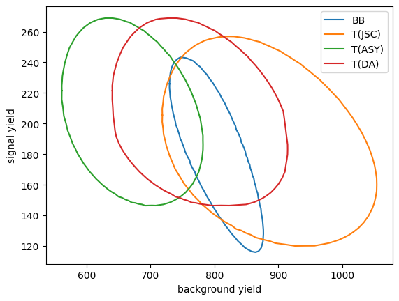
In this particular example, the BB method produces the smallest uncertainty for the background yield. The uncertainty for the signal yield is similar for all methods.
In general, the approximate methods perform well, the T(DA) method in particular is very close to the performance of the exact BB likelihood. The T(DA) method also has the advantage that it can be used with weighted data and/or weighted simulated samples.
For an in-depth comparison of the four methods, see H. Dembinski, A. Abdelmotteleb, Eur.Phys.J.C 82 (2022) 11, 1043.