Fitting a mixture of templates and parametric models

The class iminuit.cost.Template supports fitting a mixture of templates and parametric models. This is useful if some components have a simple shape like a Gaussian peak, while other components are complicated and need to be estimated from simulation or a control measurement.

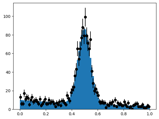
In this notebook, we demonstrate this usage. Our data consists of a Gaussian peak and exponential background. We fit the Gaussian peak with a parametric model and use a template to describe the exponential background.

from iminuit import Minuit
from iminuit.cost import Template, ExtendedBinnedNLL
from numba_stats import norm, truncexpon
import numpy as np
from matplotlib import pyplot as plt

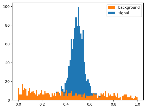
We generate the toy data.

rng = np.random.default_rng(1)

s = rng.normal(0.5, 0.05, size=1000)
b = rng.exponential(1, size=1000)
b = b[b < 1]

ns, xe = np.histogram(s, bins=100, range=(0, 1))
nb, _ = np.histogram(b, bins=xe)
n = ns + nb

plt.stairs(nb, xe, color="C1", fill=True, label="background")
plt.stairs(n, xe, baseline=nb, color="C0", fill=True, label="signal")
plt.legend();

Fitting a parametric component and a template

We now model the peaking component parametrically with a Gaussian. A template fit is an extended binned fit, so we need to provide a scaled cumulative density function like for iminuit.cost.ExtendedBinnedNLL. To obtain a background template, we generate more samples from the exponential distribution and make a histogram.

# signal model: scaled cdf of a normal distribution
def signal(xe, n, mu, sigma):
    return n * norm.cdf(xe, mu, sigma)

# background template: histogram of MC simulation
rng = np.random.default_rng(2)
b2 = rng.exponential(1, size=1000)
b2 = b2[b2 < 1]
template = np.histogram(b2, bins=xe)[0]

# fit
c = Template(n, xe, (signal, template))
m = Minuit(c, x0_n=500, x0_mu=0.5, x0_sigma=0.05, x1=100)
m.limits["x0_n", "x1", "x0_sigma"] = (0, None)
m.limits["x0_mu"] = (0, 1)
m.migrad()

Migrad
FCN = 87.01 (chi2/ndof = 0.9)		Nfcn = 194
EDM = 4.93e-05 (Goal: 0.0002)
Valid Minimum		No Parameters at limit
Below EDM threshold (goal x 10)		Below call limit
Covariance	Hesse ok	Accurate	Pos. def.	Not forced

	Name	Value	Hesse Error	Minos Error-	Minos Error+	Limit-	Limit+	Fixed
0	x0_n	990	40			0
1	x0_mu	0.4951	0.0020			0	1
2	x0_sigma	0.0484	0.0018			0
3	x1	630	40			0

	x0_n	x0_mu	x0_sigma	x1
x0_n	1.43e+03	0.000324 (0.004)	0.0185 (0.274)	-441 (-0.284)
x0_mu	0.000324 (0.004)	3.87e-06	-5.26e-08 (-0.015)	-0.000347 (-0.004)
x0_sigma	0.0185 (0.274)	-5.26e-08 (-0.015)	3.21e-06	-0.0185 (-0.251)
x1	-441 (-0.284)	-0.000347 (-0.004)	-0.0185 (-0.251)	1.69e+03

m.visualize()

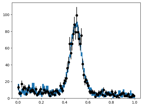
The fit succeeded and the statistical uncertainty in the template is propagated into the result. You can play with this demo and see what happens if you increase the statistic of the template.

Note: the parameters of a parametric components are prefixed with xn_ where n is the index of the component. This is to avoid name clashes between the parameter names of individual components and for clarity which parameter belongs to which component.

Extreme case: Fitting two parametric components

Although this is not recommended, you can also use the Template class with two parametric components and no template. If you are in that situation, however, it is simpler and more efficient to use iminuit.cost.ExtendedBinnedNLL. The following snipped is therefore just a proof that iminuit.cost.Template handles this limiting case as well.

# signal model: scaled cdf of a normal distribution
def signal(xe, n, mu, sigma):
    return n * norm.cdf(xe, mu, sigma)

# background model: scaled cdf a an exponential distribution
def background(xe, n, mu):
    return n * truncexpon.cdf(xe, xe[0], xe[-1], 0, mu)

# fit
c = Template(n, xe, (signal, background))
m = Minuit(c, x0_n=500, x0_mu=0.5, x0_sigma=0.05, x1_n=100, x1_mu=1)
m.limits["x0_n", "x1_n", "x0_sigma", "x1_mu"] = (0, None)
m.limits["x0_mu"] = (0, 1)
m.migrad()

Migrad
FCN = 92.87 (chi2/ndof = 1.0)		Nfcn = 190
EDM = 1.67e-05 (Goal: 0.0002)
Valid Minimum		No Parameters at limit
Below EDM threshold (goal x 10)		Below call limit
Covariance	Hesse ok	Accurate	Pos. def.	Not forced

	Name	Value	Hesse Error	Minos Error-	Minos Error+	Limit-	Limit+	Fixed
0	x0_n	990	40			0
1	x0_mu	0.4964	0.0019			0	1
2	x0_sigma	0.0487	0.0016			0
3	x1_n	629	29			0
4	x1_mu	0.97	0.14			0

	x0_n	x0_mu	x0_sigma	x1_n	x1_mu
x0_n	1.3e+03	0.000424 (0.006)	0.0123 (0.209)	-264 (-0.252)	-0.369 (-0.076)
x0_mu	0.000424 (0.006)	3.44e-06	-9.8e-08 (-0.032)	0.000293 (0.005)	-1.64e-05 (-0.065)
x0_sigma	0.0123 (0.209)	-9.8e-08 (-0.032)	2.64e-06	-0.0129 (-0.271)	-1.64e-05 (-0.075)
x1_n	-264 (-0.252)	0.000293 (0.005)	-0.0129 (-0.271)	851	0.337 (0.085)
x1_mu	-0.369 (-0.076)	-1.64e-05 (-0.065)	-1.64e-05 (-0.075)	0.337 (0.085)	0.0183

m.visualize()

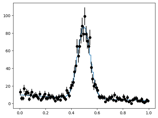
The result is identical when we fit with iminuit.cost.ExtendedBinnedNLL.

def total(xe, x0_n, x0_mu, x0_sigma, x1_n, x1_mu):
    return signal(xe, x0_n, x0_mu, x0_sigma) + background(xe, x1_n, x1_mu)

c = ExtendedBinnedNLL(n, xe, total)
m = Minuit(c, x0_n=500, x0_mu=0.5, x0_sigma=0.05, x1_n=100, x1_mu=1)
m.limits["x0_n", "x1_n", "x0_sigma", "x1_mu"] = (0, None)
m.limits["x0_mu"] = (0, 1)
m.migrad()

Migrad
FCN = 92.87 (chi2/ndof = 1.0)		Nfcn = 190
EDM = 1.67e-05 (Goal: 0.0002)
Valid Minimum		No Parameters at limit
Below EDM threshold (goal x 10)		Below call limit
Covariance	Hesse ok	Accurate	Pos. def.	Not forced

	Name	Value	Hesse Error	Minos Error-	Minos Error+	Limit-	Limit+	Fixed
0	x0_n	990	40			0
1	x0_mu	0.4964	0.0019			0	1
2	x0_sigma	0.0487	0.0016			0
3	x1_n	629	29			0
4	x1_mu	0.97	0.14			0

	x0_n	x0_mu	x0_sigma	x1_n	x1_mu
x0_n	1.3e+03	0.000424 (0.006)	0.0123 (0.209)	-264 (-0.252)	-0.369 (-0.076)
x0_mu	0.000424 (0.006)	3.44e-06	-9.8e-08 (-0.032)	0.000293 (0.005)	-1.64e-05 (-0.065)
x0_sigma	0.0123 (0.209)	-9.8e-08 (-0.032)	2.64e-06	-0.0129 (-0.271)	-1.64e-05 (-0.075)
x1_n	-264 (-0.252)	0.000293 (0.005)	-0.0129 (-0.271)	851	0.337 (0.085)
x1_mu	-0.369 (-0.076)	-1.64e-05 (-0.065)	-1.64e-05 (-0.075)	0.337 (0.085)	0.0183

m.visualize()