Reference

Quick Summary

These methods and properties you will probably use a lot:

`Minuit`(fcn, *args[, grad, name])	Function minimizer and error computer.
`Minuit.migrad`([ncall, iterate])	Run Migrad minimization.
`Minuit.hesse`([ncall])	Run Hesse algorithm to compute asymptotic errors.
`Minuit.minos`(*parameters[, cl, ncall])	Run Minos algorithm to compute confidence intervals.
`Minuit.values`	Access parameter values via an array-like view.
`Minuit.errors`	Access parameter parabolic errors via an array-like view.
`Minuit.merrors`	Return a dict-like with Minos data objects.
`Minuit.fixed`	Access whether parameters are fixed via an array-like view.
`Minuit.limits`	Access parameter limits via a array-like view.
`Minuit.covariance`	Return covariance matrix.
`Minuit.valid`	Return True if the function minimum is valid.
`Minuit.accurate`	Return True if the covariance matrix is accurate.
`Minuit.fval`	Get function value at minimum.
`Minuit.nfit`	Get number of fitted parameters (fixed parameters not counted).
`Minuit.mnprofile`(vname, *[, size, bound, ...])	Get Minos profile over a specified interval.
`Minuit.draw_mnprofile`(vname, *[, band, text])	Draw Minos profile over a specified interval (requires matplotlib).

Minuit

class iminuit.Minuit(fcn: Callable, *args: float | Sequence[float], grad: Callable | None = None, name: Collection[str] | None = None, **kwds: float)

Function minimizer and error computer.

Initialize Minuit object.

This does not start the minimization or perform any other work yet. Algorithms are started by calling the corresponding methods.

Parameters:

fcn – Function to minimize. See notes for details on what kind of functions are accepted.
*args – Starting values for the minimization as positional arguments. See notes for details on how to set starting values.
grad – Function that calculates the gradient and returns an iterable object with one entry for each parameter, which is the derivative for that parameter. If None (default), Minuit will calculate the gradient numerically.
name – If it is set, it overrides iminuit’s function signature detection.
**kwds – Starting values for the minimization as keyword arguments. See notes for details on how to set starting values.

Notes

Callables

By default, Minuit assumes that the callable fcn behaves like chi-square function, meaning that the function minimum in repeated identical random experiments is chi-square distributed up to an arbitrary additive constant. This is important for the correct error calculation. If fcn returns a log-likelihood, one should multiply the result with -2 to adapt it. If the function returns the negated log-likelihood, one can alternatively set the attribute fcn.errordef = Minuit.LIKELIHOOD or Minuit.errordef = Minuit.LIKELIHOOD after initialization to make Minuit calculate errors properly.

Minuit reads the function signature of fcn to detect the number and names of the function parameters. Two kinds of function signatures are understood.

Function with positional arguments.
The function has positional arguments, one for each fit parameter. Example:
def fcn(a, b, c): ...
The parameters a, b, c must accept a real number.

iminuit automatically detects the parameters names in this case. More information about how the function signature is detected can be found in iminuit.util.describe().
Function with arguments passed as a single Numpy array.
The function has a single argument which is a Numpy array. Example:
def fcn_np(x): ...
To use this form, starting values need to be passed to Minuit in form as an array-like type, e.g. a numpy array, tuple or list. For more details, see “Parameter Keyword Arguments” further down.

In some cases, the detection fails, for example, for a function like this:

def difficult_fcn(*args): ...

To use such a function, set the name keyword as described further below.

Parameter initialization

Initial values for the minimization can be set with positional arguments or via keywords. This is best explained through an example:

def fcn(x, y):
    return (x - 2) ** 2 + (y - 3) ** 2

The following ways of passing starting values are equivalent:

Minuit(fcn, x=1, y=2)
Minuit(fcn, y=2, x=1) # order is irrelevant when keywords are used ...
Minuit(fcn, 1, 2)     # ... but here the order matters

Positional arguments can also be used if the function has no signature:

def fcn_no_sig(*args):
    # ...

Minuit(fcn_no_sig, 1, 2)

If the arguments are explicitly named with the name keyword described further below, keywords can be used for initialization:

Minuit(fcn_no_sig, x=1, y=2, name=("x", "y"))  # this also works

If the function accepts a single Numpy array, then the initial values must be passed as a single array-like object:

def fcn_np(x):
    return (x[0] - 2) ** 2 + (x[1] - 3) ** 2

Minuit(fcn_np, (1, 2))

Setting the values with keywords is not possible in this case. Minuit deduces the number of parameters from the length of the initialization sequence.

contour(x: int | str, y: int | str, *, size: int = 50, bound: float | Iterable[Tuple[float, float]] = 2, grid: Tuple[Sequence, Sequence] | None = None, subtract_min: bool = False) → Tuple[ndarray, ndarray, ndarray]

Get a 2D contour of the function around the minimum.

It computes the contour via a function scan over two parameters, while keeping all other parameters fixed. The related mncontour() works differently: for each pair of parameter values in the scan, it minimises the function with the respect to all other parameters.

This method is useful to inspect the function near the minimum to detect issues (the contours should look smooth). It is not a confidence region unless the function only has two parameters. Use mncontour() to compute confidence regions.

Parameters:

x (int or str) – First parameter for scan.
y (int or str) – Second parameter for scan.
size (int or tuple of int, optional) – Number of scanning points per parameter (Default: 50). A tuple is interpreted as the number of scanning points per parameter. Ignored if grid is set.
bound (float or tuple of floats, optional) – If bound is 2x2 array, [[v1min,v1max],[v2min,v2max]]. If bound is a number, it specifies how many \(\sigma\) symmetrically from minimum (minimum+- bound*:math:sigma). (Default: 2). Ignored if grid is set.
grid (tuple of array-like, optional) – Grid points to scan over. If grid is set, size and bound are ignored.
subtract_min – Subtract minimum from return values (Default: False).

Returns:

array of float – Parameter values of first parameter.
array of float – Parameter values of second parameter.
2D array of float – Function values.

See also

mncontour, mnprofile

draw_contour(x: int | str, y: int | str, **kwargs) → Tuple[ndarray, ndarray, ndarray]

Draw 2D contour around minimum (requires matplotlib).

See contour() for details on parameters and interpretation. Please also read the docs of mncontour() to understand the difference between the two.

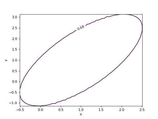
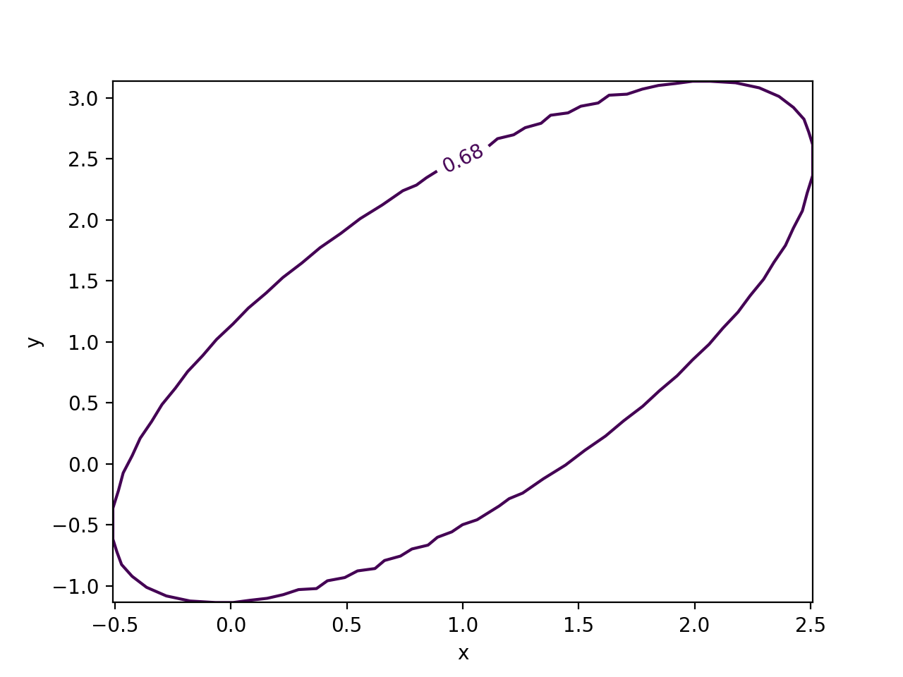
draw_mncontour(x: int | str, y: int | str, *, cl: float | Sequence[float] | None = None, size: int = 100, interpolated: int = 0, experimental: bool = False) → Any

Draw 2D Minos confidence region (requires matplotlib).

See mncontour() for details on the interpretation of the region and for the parameters accepted by this function.

Examples

from iminuit import Minuit

def cost(x, y, z):
    return (x - 1) ** 2 + (y - x) ** 2 + (z - 2) ** 2

cost.errordef = Minuit.LEAST_SQUARES

m = Minuit(cost, x=0, y=0, z=0)
m.migrad()
m.draw_mncontour("x", "y")

(Source code, png, hires.png, pdf)

Returns:: Instance of a ContourSet class from matplot.contour.
Return type:: ContourSet

See also

mncontour

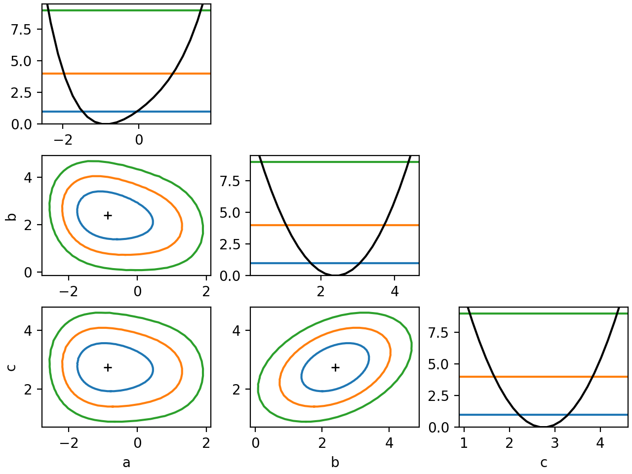
draw_mnmatrix(*, cl: float | Sequence[float] | None = None, size: int = 100, experimental: bool = False, figsize=None) → Any

Draw matrix of Minos scans (requires matplotlib).

This draws a matrix of Minos likelihood scans, meaning that the likelihood is minimized with respect to the parameters that are not scanned over. The diagonal cells of the matrix show the 1D scan, the off-diagonal cells show 2D scans for all unique pairs of parameters. The 2D scans show confidence regions. See mncontour() for details on the interpretation of these regions.

Parameters:

cl (float or array-like of floats, optional) – See mncontour().
size (int, optional) – See mncontour()
experimental (bool, optional) – See mncontour()
figsize ((float, float) or None, optional) – Width and height of figure in inches.

Examples

from iminuit import Minuit


def cost(a, b, c):
    return (
        a**2
        + 0.25 * a**4
        + a * b
        + ((b - 1) / 0.6) ** 2
        - 2.5 * b * c
        + ((c - 2) / 0.5) ** 2
    )


m = Minuit(cost, 1, 1, 1)
m.migrad()

m.draw_mnmatrix(cl=[1, 2, 3])

(Source code, png, hires.png, pdf)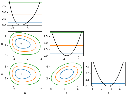

Returns:: Figure and axes instances generated by matplotlib.
Return type:: fig, ax

See also

mncontour

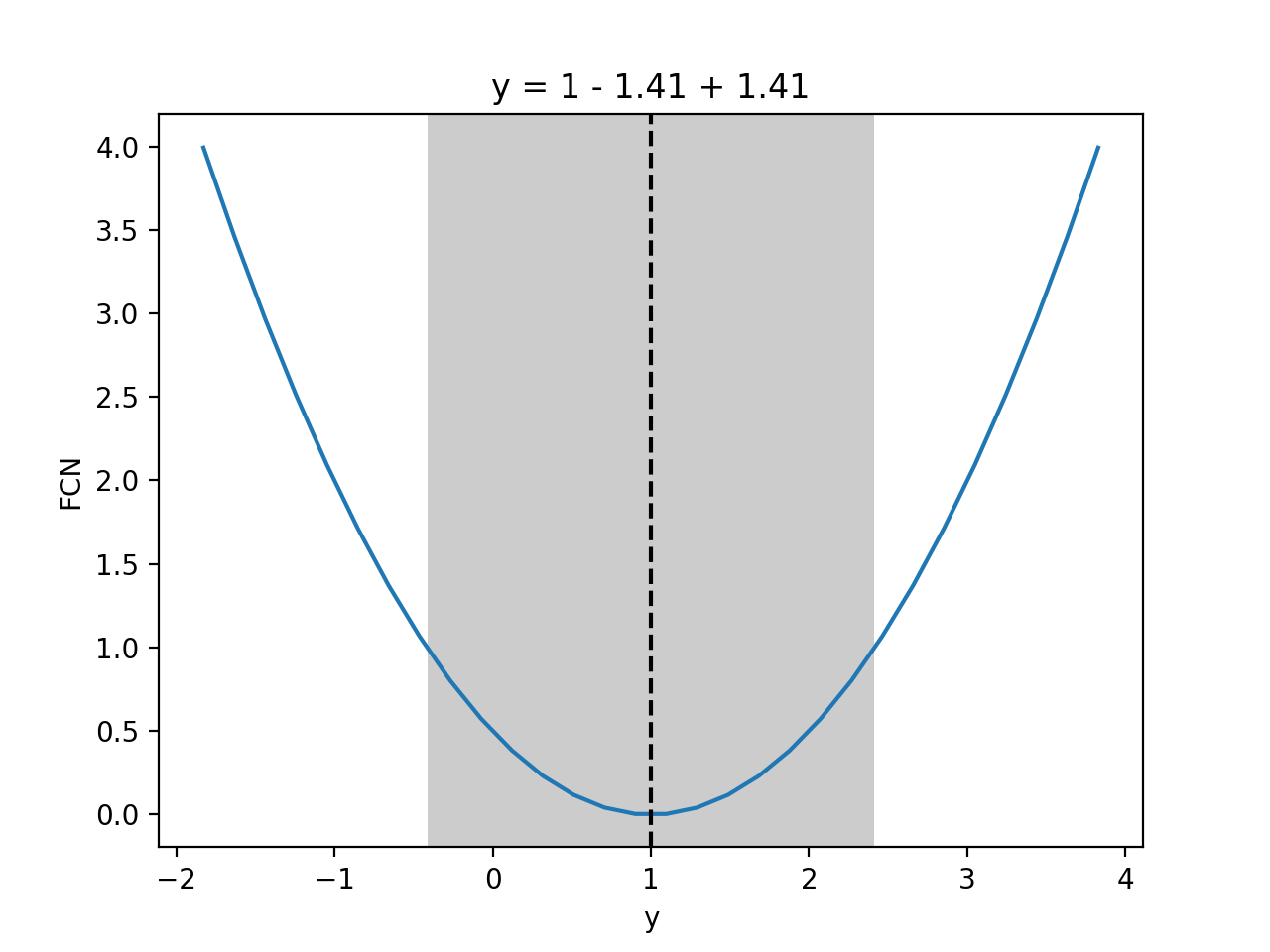
draw_mnprofile(vname: int | str, *, band: bool = True, text: bool = True, **kwargs) → Tuple[ndarray, ndarray]

Draw Minos profile over a specified interval (requires matplotlib).

See mnprofile() for details and shared arguments. The following additional arguments are accepted.

Parameters:

band (bool, optional) – If true, show a band to indicate the Hesse error interval (Default: True).
text (bool, optional) – If true, show text a title with the function value and the Hesse error (Default: True).

Examples

from iminuit import Minuit

def cost(x, y, z):
    return (x - 1) ** 2 + (y - x) ** 2 + (z - 2) ** 2

cost.errordef = Minuit.LEAST_SQUARES

m = Minuit(cost, x=0, y=0, z=0)
m.migrad()
m.draw_mnprofile("y")

(Source code, png, hires.png, pdf)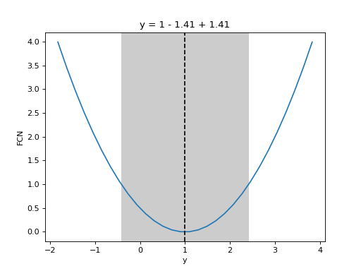

See also

mnprofile, profile, draw_profile

draw_profile(vname: int | str, *, band: bool = True, text: bool = True, **kwargs) → Tuple[ndarray, ndarray]

Draw 1D cost function profile over a range (requires matplotlib).

See profile() for details and shared arguments. The following additional arguments are accepted.

Parameters:

band (bool, optional) – If true, show a band to indicate the Hesse error interval (Default: True).
text (bool, optional) – If true, show text a title with the function value and the Hesse error (Default: True).

Fix parameter and set it to value.

This is a convenience function to fix a parameter and set it to a value at the same time. It is equivalent to calling fixed and values.

Parameters:

key (int, str, slice, list of int or str) – Key, which can be an index, name, slice, or list of indices or names.
value (float or sequence of float) – Value(s) assigned to key(s).

Return type:

self

hesse(ncall: int | None = None) → Minuit

Run Hesse algorithm to compute asymptotic errors.

The Hesse method estimates the covariance matrix by inverting the matrix of second derivatives (Hesse matrix) at the minimum. To get parameters correlations, you need to use this. The Minos algorithm is another way to estimate parameter uncertainties, see minos().

Parameters:: ncall – Approximate upper limit for the number of calls made by the Hesse algorithm. If set to None, use the adaptive heuristic from the Minuit2 library (Default: None).

Notes

The covariance matrix is asymptotically (in large samples) valid. By valid we mean that confidence intervals constructed from the errors contain the true value with a well-known coverage probability (68 % for each interval). In finite samples, this is likely to be true if your cost function looks like a hyperparabola around the minimum.

In practice, the errors very likely have correct coverage if the results from Minos and Hesse methods agree. It is possible to construct artifical functions where this rule is violated, but in practice it should always work.

See also

minos

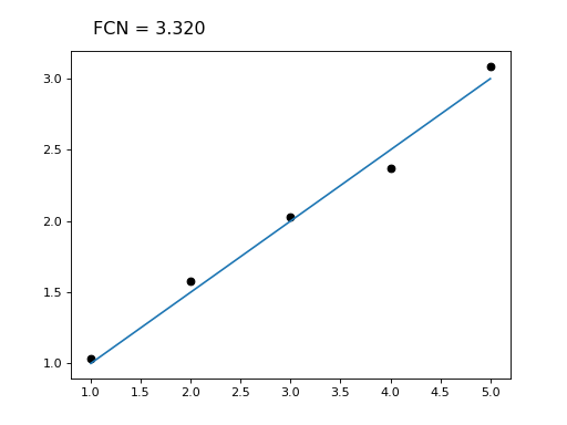
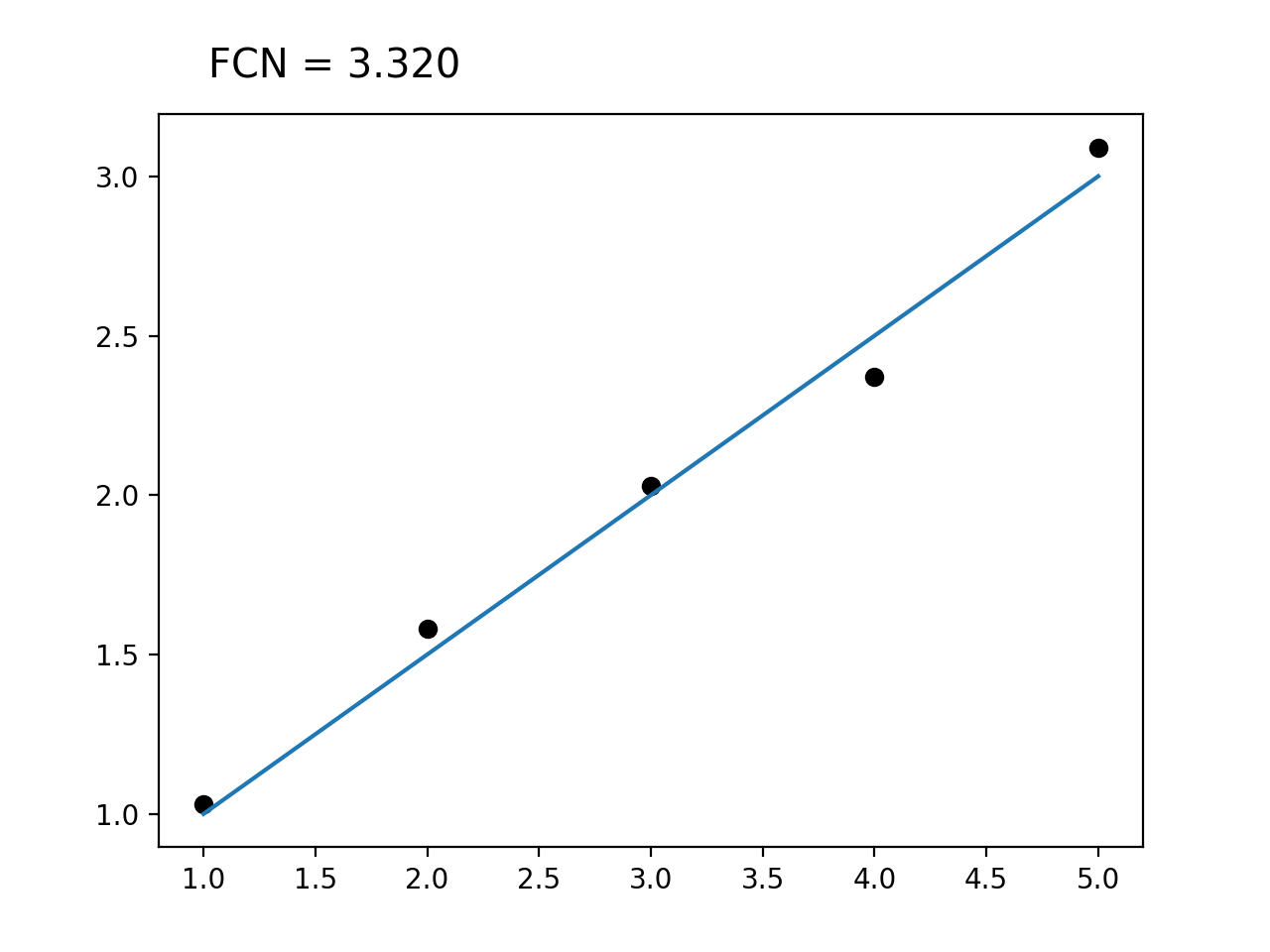
interactive(plot: Callable | None = None, raise_on_exception=False, **kwargs)

Return fitting widget (requires ipywidgets, IPython, matplotlib).

A fitting widget is returned which can be displayed and manipulated in a Jupyter notebook to find good starting parameters and to debug the fit.

Parameters:

plot (Callable, optional) – To visualize the fit, interactive tries to access the visualize method on the cost function, which accepts the current model parameters as an array-like and potentially further keyword arguments, and draws a visualization into the current matplotlib axes. If the cost function does not provide a visualize method or if you want to override it, pass the function here.
raise_on_exception (bool, optional) – The default is to catch exceptions in the plot function and convert them into a plotted message. In unit tests, raise_on_exception should be set to True to allow detecting errors.
**kwargs – Any other keyword arguments are forwarded to the plot function.

Examples

from iminuit import Minuit, cost
import numpy as np
from matplotlib import pyplot as plt


# custom visualization, x and y are taken from outer scope
def viz(args):
    plt.plot(x, y, "ok")
    xm = np.linspace(x[0], x[-1], 100)
    plt.plot(xm, model(xm, *args))


def model(x, a, b):
    return a + b * x


x = np.array([1, 2, 3, 4, 5])
y = np.array([1.03, 1.58, 2.03, 2.37, 3.09])
c = cost.LeastSquares(x, y, 0.1, model)
m = Minuit(c, 0.5, 0.5)
m.interactive(viz)  # calling m.interactive() uses LeastSquares.visualize

(Source code, png, hires.png, pdf)

migrad(ncall: int | None = None, iterate: int = 5) → Minuit

Run Migrad minimization.

Migrad from the Minuit2 library is a robust minimisation algorithm which earned its reputation in 40+ years of almost exclusive usage in high-energy physics. How Migrad works is described in the Minuit paper. It uses first and approximate second derivatives to achieve quadratic convergence near the minimum.

Parameters:

ncall – Approximate maximum number of calls before minimization will be aborted. If set to None, use the adaptive heuristic from the Minuit2 library (Default: None). Note: The limit may be slightly violated, because the condition is checked only after a full iteration of the algorithm, which usually performs several function calls.
iterate – Automatically call Migrad up to N times if convergence was not reached (Default: 5). This simple heuristic makes Migrad converge more often even if the numerical precision of the cost function is low. Setting this to 1 disables the feature.

See also

simplex, scan

minos(*parameters: int | str, cl: float | None = None, ncall: int | None = None) → Minuit

Run Minos algorithm to compute confidence intervals.

The Minos algorithm uses the profile likelihood method to compute (generally asymmetric) confidence intervals. It scans the negative log-likelihood or (equivalently) the least-squares cost function around the minimum to construct a confidence interval.

Parameters:

*parameters – Names of parameters to generate Minos errors for. If no positional arguments are given, Minos is run for each parameter.
cl (float or None, optional) – Confidence level for the confidence interval. If not set or None, a standard 68.3 % confidence interval is produced. Setting this to another value requires the scipy module to be installed. If 0 < cl < 1, the value is interpreted as the confidence level (a probability). If cl >= 1, it is interpreted as number of standard deviations. For example, cl=3 produces a 3 sigma interval. Values other than 0.68, 0.9, 0.95, 0.99, 1, 2, 3, 4, 5 require the scipy module.
ncall (int or None, optional) – Limit the number of calls made by Minos. If None, an adaptive internal heuristic of the Minuit2 library is used (Default: None).

Notes

Asymptotically (large samples), the Minos interval has a coverage probability equal to the given confidence level. The coverage probability is the probability for the interval to contain the true value in repeated identical experiments.

The interval is invariant to transformations and thus not distorted by parameter limits, unless the limits intersect with the confidence interval. As a rule-of-thumb: when the confidence intervals computed with the Hesse and Minos algorithms differ strongly, the Minos intervals are preferred. Otherwise, Hesse intervals are preferred.

Running Minos is computationally expensive when there are many fit parameters. Effectively, it scans over one parameter in small steps and runs a full minimisation for all other parameters of the cost function for each scan point. This requires many more function evaluations than running the Hesse algorithm.

mncontour(x: int | str, y: int | str, *, cl: float | None = None, size: int = 100, interpolated: int = 0, experimental: bool = False) → ndarray

Get 2D Minos confidence region.

This scans over two parameters and minimises all other free parameters for each scan point. This scan produces a statistical confidence region according to the profile likelihood method with a confidence level cl, which is asymptotically equal to the coverage probability of the confidence region.

The calculation is expensive since a numerical minimisation has to be performed at various points.

Parameters:

x (str) – Variable name of the first parameter.
y (str) – Variable name of the second parameter.
cl (float or None, optional) – Confidence level of the contour. If not set or None, a standard 68 % contour is computed (default). If 0 < cl < 1, the value is interpreted as the confidence level (a probability). If cl >= 1, it is interpreted as number of standard deviations. For example, cl=3 produces a 3 sigma contour. Values other than 0.68, 0.9, 0.95, 0.99, 1, 2, 3, 4, 5 require the scipy module.
size (int, optional) – Number of points on the contour to find (default: 100). Increasing this makes the contour smoother, but requires more computation time.
interpolated (int, optional) – Number of interpolated points on the contour (default: 0). If you set this to a value larger than size, cubic spline interpolation is used to generate a smoother curve and the interpolated coordinates are returned. Values smaller than size are ignored. Good results can be obtained with size=20, interpolated=200. This requires scipy.
experimental (bool, optional) – If true, use experimental implementation to compute contour, otherwise use MnContour from the Minuit2 library. The experimental implementation was found to succeed in cases where MnContour produced no reasonable result, but is slower and not yet well tested in practice. Use with caution and report back any issues via Github.

Returns:

Contour points of the form [[x1, y1]…[xn, yn]]. Note that N = size + 1, the last point [xn, yn] is identical to [x1, y1]. This makes it easier to draw a closed contour.

Return type:

array of float (N x 2)

See also

contour, mnprofile

mnprofile(vname: int | str, *, size: int = 30, bound: float | UserBound = 2, grid: Sequence[float] | None = None, subtract_min: bool = False) → Tuple[ndarray, ndarray, ndarray]

Get Minos profile over a specified interval.

Scans over one parameter and minimises the function with respect to all other parameters for each scan point.

Parameters:

vname (int or str) – Parameter to scan over.
size (int, optional) – Number of scanning points (Default: 100). Ignored if grid is set.
bound (tuple of float or float, optional) – If bound is tuple, (left, right) scanning bound. If bound is a number, it specifies an interval of N \(\sigma\) symmetrically around the minimum (Default: 2). Ignored if grid is set.
grid (array-like, optional) – Parameter values on which to compute the profile. If grid is set, size and bound are ignored.
subtract_min (bool, optional) – If true, subtract offset so that smallest value is zero (Default: False).

Returns:

array of float – Parameter values where the profile was computed.
array of float – Profile values.
array of bool – Whether minimisation in each point succeeded or not.

profile(vname: int | str, *, size: int = 100, bound: float | UserBound = 2, grid: Sequence[float] | None = None, subtract_min: bool = False) → Tuple[ndarray, ndarray]

Calculate 1D cost function profile over a range.

A 1D scan of the cost function around the minimum, useful to inspect the minimum. For a fit with several free parameters this is not the same as the Minos profile computed by mncontour().

Parameters:

vname (int or str) – Parameter to scan over.
size (int, optional) – Number of scanning points (Default: 100). Ignored if grid is set.
bound (tuple of float or float, optional) – If bound is tuple, (left, right) scanning bound. If bound is a number, it specifies an interval of N \(\sigma\) symmetrically around the minimum (Default: 2). Ignored if grid is set.
grid (array-like, optional) – Parameter values on which to compute the profile. If grid is set, size and bound are ignored.
subtract_min (bool, optional) – If true, subtract offset so that smallest value is zero (Default: False).

Returns:

array of float – Parameter values.
array of float – Function values.

See also

mnprofile

reset() → Minuit

Reset minimization state to initial state.

Leaves strategy, precision, tol, errordef, print_level unchanged.

scan(ncall: int | None = None) → Minuit

Brute-force minimization.

Scans the function on a regular hypercube grid, whose bounds are defined either by parameter limits if present or by Minuit.values +/- Minuit.errors. Minuit.errors are initialized to very small values by default, too small for this scan. They should be increased before running scan or limits should be set. The scan evaluates the function exactly at the limit boundary, so the function should be defined there.

Parameters:: ncall – Approximate number of function calls to spend on the scan. The actual number will be close to this, the scan uses ncall^(1/npar) steps per cube dimension. If no value is given, a heuristic is used to set ncall.

Notes

The scan can return an invalid minimum, this is not a cause for alarm. It just minimizes the cost function, the EDM value is only computed after the scan found a best point. If the best point still has a bad EDM value, the minimum is considered invalid. But even if it is considered valid, it is probably not accurate, since the tolerance is very lax. One should always run migrad() after the scan.

This implementation here does a full scan of the hypercube in Python. Originally, this was supposed to use MnScan from C++ Minuit2, but MnScan is unsuitable. It does a 1D scan with 41 steps (not configurable) for each parameter in sequence, so it is not actually scanning the full hypercube. It first scans one parameter, then starts the scan of the second parameter from the best value of the first and so on. This fails easily when the parameters are correlated.

Minimize with SciPy algorithms.

Parameters:

method (str or Callable, optional) – Which scipy method to use.
ncall (int, optional) – Function call limit.
hess (Callable, optional) – Function that computes the Hessian matrix. It must use the exact same calling conversion as the original fcn (several arguments which are numbers or a single array argument).
hessp (Callable, optional) – Function that computes the product of the Hessian matrix with a vector. It must use the same calling conversion as the original fcn (several arguments which are numbers or a single array argument) and end with another argument which is an arbitrary vector.
constraints (scipy.optimize.LinearConstraint or) – scipy.optimize.NonlinearConstraint, optional Linear or non-linear constraints, see docs of scipy.optimize.minimize() look for the constraints parameter. The function used in the constraint must use the exact same calling convention as the original fcn, see hess parameter for details. No parameters may be omitted in the signature, even if those parameters are not used in the constraint.

Notes

The call limit may be violated since many algorithms checks the call limit only after a full iteraction of their algorithm, which consists of several function calls. Some algorithms do not check the number of function calls at all, in this case the call limit acts on the number of iterations of the algorithm. This issue should be fixed in scipy.

The SciPy minimizers use their own internal rule for convergence. The EDM criterion is evaluated only after the original algorithm already stopped. This means that usually SciPy minimizers will use more iterations than Migrad and the tolerance tol has no effect on SciPy minimizers.

simplex(ncall: int | None = None) → Minuit

Run Simplex minimization.

Simplex from the Minuit2 C++ library is a variant of the Nelder-Mead algorithm to find the minimum of a function. It does not make use of derivatives. The Wikipedia has a good article on the Nelder-Mead method.

Parameters:: ncall – Approximate maximum number of calls before minimization will be aborted. If set to None, use the adaptive heuristic from the Minuit2 library (Default: None). Note: The limit may be slightly violated, because the condition is checked only after a full iteration of the algorithm, which usually performs several function calls.

Notes

The Simplex method usually converges more slowly than Migrad, but performs better in certain cases, the Rosenbrock function is a notable example. Unlike Migrad, the Simplex method does not have quadratic convergence near the minimum, so it is a good approach to run Migrad after Simplex to obtain an accurate solution in fewer steps. Simplex may also be useful to get close to the minimum from an unsuitable starting point.

The convergence criterion for Simplex is also based on EDM, but the threshold is much more lax than that of Migrad (see Minuit.tol for details). This was made so that Simplex stops early when getting near the minimum, to give the user a chance to switch to the more efficient Migrad algorithm to finish the minimization. Early stopping can be avoided by setting Minuit.tol to an accordingly smaller value, however.

visualize(plot: Callable | None = None, **kwargs)

Visualize agreement of current model with data (requires matplotlib).

This generates a plot of the data/model agreement, using the current parameter values, if the likelihood function supports this, otherwise AttributeError is raised.

Parameters:

plot (Callable, optional) – This function tries to call the visualize method on the cost function, which accepts the current model parameters as an array-like and potentially further keyword arguments, and draws a visualization into the current matplotlib axes. If the cost function does not provide a visualize method or if you want to override it, pass the function here.
kwargs – Other keyword arguments are forwarded to the plot function.

LEAST_SQUARES = 1.0

LIKELIHOOD = 0.5

property accurate: bool

Return True if the covariance matrix is accurate.

This is an alias for iminuit.util.FMin.has_accurate_covar.

See also

util.FMin

property covariance: Matrix | None

Return covariance matrix.

The square-root of the diagonal elements of the covariance matrix correspond to a standard deviation for each parameter with 68 % coverage probability in the asymptotic limit (large samples). To get k standard deviations, multiply the covariance matrix with k^2.

The submatrix formed by two parameters describes an ellipse. The asymptotic coverage probabilty of the standard ellipse is lower than 68 %. It can be computed from the \(\chi^2\) distribution with 2 degrees of freedom. In general, to obtain a (hyper-)ellipsoid with coverage probability CL, one has to multiply the submatrix of the corresponding k parameters with a factor. For k = 1,2,3 and CL = 0.99

from scipy.stats import chi2

chi2(1).ppf(0.99) # 6.63...
chi2(2).ppf(0.99) # 9.21...
chi2(3).ppf(0.99) # 11.3...

See also

util.Matrix

property errordef: float

Access FCN increment above minimum that corresponds to one standard deviation.

Default value is 1.0. errordef should be 1.0 for a least-squares cost function and 0.5 for a negative log-likelihood function. See section 1.5.1 on page 6 of the MINUIT2 User's Guide. This parameter is also called UP in MINUIT documents.

To make user code more readable, we provided two named constants:

m_lsq = Minuit(a_least_squares_function)
m_lsq.errordef = Minuit.LEAST_SQUARES  # == 1

m_nll = Minuit(a_likelihood_function)
m_nll.errordef = Minuit.LIKELIHOOD     # == 0.5

property errors: ErrorView

Access parameter parabolic errors via an array-like view.

Like values, but instead of reading or writing the values, you read or write the errors (which double as step sizes for MINUITs numerical gradient estimation). Only positive values are accepted when assigning to errors.

See also

values, fixed, limits

property fcn: FCN: Get cost function (usually a least-squares or likelihood function).

property fixed: FixedView

Access whether parameters are fixed via an array-like view.

Use to read or write the fixation state of a parameter based on the parameter index or the parameter name as a string. If you change the state and run migrad(), hesse(), or minos(), the new state is used.

In case of complex fits, it can help to fix some parameters first and only minimize the function with respect to the other parameters, then release the fixed parameters and minimize again starting from that state.

See also

values, errors, limits

property fmin: FMin | None: Get function minimum data object.

See also

util.FMin

property fval: float | None

Get function value at minimum.

This is an alias for iminuit.util.FMin.fval.

See also

util.FMin

property grad: Callable[[ndarray], ndarray]: Get gradient function of the cost function.

property init_params: Params: Get list of current parameter data objects set to the initial fit state.

See also

params, util.Params

property limits: LimitView

Access parameter limits via a array-like view.

Use to read or write the limits of a parameter based on the parameter index or the parameter name as a string. If you change the limits and run migrad(), hesse(), or minos(), the new state is used.

In case of complex fits, it can help to limit some parameters first, run Migrad, then remove the limits and run Migrad again. Limits will bias the result only if the best fit value is outside the limits, not if it is inside. Limits will affect the estimated Hesse uncertainties if the parameter is close to a limit. They do not affect the Minos uncertainties, because those are invariant to transformations and limits are implemented via a variable transformation.

See also

values, errors, fixed

property merrors: MErrors

Return a dict-like with Minos data objects.

The Minos data objects contain the full status information of the Minos run.

See also

util.MError, util.MErrors

property ndof: int

Get number of degrees of freedom if cost function supports this.

To support this feature, the cost function has to report the number of data points with a property called ndata. Unbinned cost functions should return infinity.

property nfcn: int: Get total number of function calls.

property nfit: int: Get number of fitted parameters (fixed parameters not counted).

property ngrad: int: Get total number of gradient calls.

property npar: int: Get number of parameters.

property parameters: Tuple[str, ...]

Get tuple of parameter names.

This is an alias for pos2var.

property params: Params: Get list of current parameter data objects.

See also

init_params, util.Params

property pos2var: Tuple[str, ...]: Map variable index to name.

property precision: float | None

Access estimated precision of the cost function.

Default: None. If set to None, Minuit assumes the cost function is computed in double precision. If the precision of the cost function is lower (because it computes in single precision, for example) set this to some multiple of the smallest relative change of a parameter that still changes the function.

property print_level: int

Access current print level.

You can assign an integer:

0: quiet (default)
1: print minimal debug messages to terminal
2: print more debug messages to terminal
3: print even more debug messages to terminal

Warning

Setting print_level has the unwanted side-effect of setting the level globally for all Minuit instances in the current Python session.

property strategy: MnStrategy

Access current minimization strategy.

You can assign an integer:

0: Fast. Does not check a user-provided gradient. Does not improve Hesse matrix at minimum. Extra call to hesse() after migrad() is always needed for good error estimates. If you pass a user-provided gradient to MINUIT, convergence is faster.
1: Default. Checks user-provided gradient against numerical gradient. Checks and usually improves Hesse matrix at minimum. Extra call to hesse() after migrad() is usually superfluous. If you pass a user-provided gradient to MINUIT, convergence is slower.
2: Careful. Like 1, but does extra checks of intermediate Hessian matrix during minimization. The effect in benchmarks is a somewhat improved accuracy at the cost of more function evaluations. A similar effect can be achieved by reducing the tolerance tol for convergence at any strategy level.

property throw_nan: bool

Access whether to raise runtime error if the function evaluates to NaN.

If you set this to True, an error is raised whenever the function evaluates to NaN.

property tol: float

Access tolerance for convergence with the EDM criterion.

Minuit detects converge with the EDM criterion. EDM stands for Estimated Distance to Minimum, it is mathematically described in the MINUIT paper. The EDM criterion is well suited for statistical cost functions, since it stops the minimization when parameter improvements become small compared to parameter uncertainties.

The convergence is detected when edm < edm_max, where edm_max is calculated as

Migrad: edm_max = 0.002 * tol * errordef

Simplex: edm_max = tol * errordef

Users can set tol (default: 0.1) to a different value to either speed up convergence at the cost of a larger error on the fitted parameters and possibly invalid estimates for parameter uncertainties or smaller values to get more accurate parameter values, although this should never be necessary as the default is fine.

If the tolerance is set to a very small value or zero, Minuit will use an internal lower limit for the tolerance. To restore the default use, one can assign None.

Under some circumstances, Migrad is allowed to violate edm_max by a factor of 10. Users should not try to detect convergence by comparing edm with edm_max, but query iminuit.util.FMin.is_above_max_edm.

property valid: bool

Return True if the function minimum is valid.

This is an alias for iminuit.util.FMin.is_valid.

See also

util.FMin

property values: ValueView

Access parameter values via an array-like view.

Use to read or write current parameter values based on the parameter index or the parameter name as a string. If you change a parameter value and run migrad(), the minimization will start from that value, similar for hesse() and minos().

See also

errors, fixed, limits

property var2pos: Dict[str, int]: Map variable name to index.

Scipy-like interface

iminuit.minimize(fun, x0, args=(), method='migrad', jac=None, hess=None, hessp=None, bounds=None, constraints=None, tol=None, callback=None, options=None)

Interface to MIGRAD using the scipy.optimize.minimize API.

This function provides the same interface as scipy.optimize.minimize. If you are familiar with the latter, this allows you to use Minuit with a quick start. Eventually, you still may want to learn the interface of the Minuit class, as it provides more functionality if you are interested in parameter uncertainties.

For a general description of the arguments of this function, see scipy.optimize.minimize. We list only a few in the following.

Parameters:

method (str) – Allowed values are “migrad” or “simplex”. Default: “migrad”.
options (dict) – Can be used to pass special settings to Minuit. All are optional. The following options are supported. disp (bool): Set to true to print convergence messages. Default: False. stra (int): Minuit strategy (0: fast/inaccurate, 1: balanced, 2: slow/accurate). Default: 1. maxfun (int): Maximum allowed number of iterations. Default: None. maxfev (int): Deprecated alias for maxfun. eps (sequence): Initial step size to numerical compute derivative. Minuit automatically refines this in subsequent iterations and is very insensitive to the initial choice. Default: 1.

Returns:

Dict with attribute access that holds the result. It contains the following lists of fields. x (ndarray): Solution of optimization. fun (float): Value of objective function at minimum. message (str): Description of cause of termination. hess_inv (ndarray): Inverse of Hesse matrix at minimum (may not be exact). nfev (int): Number of function evaluations. njev (int): Number of jacobian evaluations. minuit (Minuit): Minuit object internally used to do the minimization. Use this to extract more information about the parameter errors.

Return type:

OptimizeResult

Cost functions

Standard cost functions to minimize for statistical fits.

We provide these for convenience, so that you do not have to write your own for standard fits. The cost functions optionally use Numba to accelerate some calculations, if Numba is installed.

What to use when

Fit a normalised probability density to data
- Data are not binned: UnbinnedNLL
- Data are binned: BinnedNLL, also supports histogram of weighted samples
Fit a density to data, density is not normalised
- Data are not binned: ExtendedUnbinnedNLL
- Data are binned: ExtendedBinnedNLL, also supports histogram of weighted samples
Fit a template to binned data with bin-wise uncertainties on the template: Template, which also supports weighted data and weighted templates
Fit of a function f(x) to (x, y, yerror) pairs with normal-distributed fluctuations. x is one- or multi-dimensional, y is one-dimensional.
- y values contain no outliers: LeastSquares
- y values contain outliers: LeastSquares with loss function set to “soft_l1”
Include constraints from external fits or apply regularisation: NormalConstraint

Combining cost functions

All cost functions can be added, which generates a new combined cost function. Parameters with the same name are shared between component cost functions. Use this to constrain one or several parameters with different data sets and using different statistical models for each data set. Gaussian penalty terms can also be added to the cost function to introduce external knowledge about a parameter.

Model parameter limits

The Minuit algorithms support box constrains in parameter space. A user-defined model can declare that a parameter is only valid over an interval on the real line with the Annotated type annotation, see iminuit.Minuit for details. A typical example is the sigma parameter of a normal distribution, which must be positive. The cost functions defined here propagate this information to iminuit.Minuit.

Note: The Template declares that the template amplitudes must be non-negative, which is usually the right choice, however, it may be desirable to fit templates which can have negative amplitudes. To achieve this, simply reset the limits with iminuit.Minuit.limits after creating the Minuit instance.

Notes

The cost functions defined here have been optimized with knowledge about implementation details of Minuit to give the highest accucary and the most robust results, so they should perform well. If you have trouble with your own implementations, try these.

The binned versions of the log-likelihood fits support weighted samples. For each bin of the histogram, the sum of weights and the sum of squared weights is needed then, see class documentation for details.

Binned negative log-likelihood.

Use this if only the shape of the fitted PDF is of interest and the data is binned. This cost function works with normal and weighted histograms. The histogram can be one- or multi-dimensional.

The cost function has a minimum value that is asymptotically chi2-distributed. It is constructed from the log-likelihood assuming a multivariate-normal distribution and using the saturated model as a reference.

Initialize cost function with data and model.

Parameters:

n (array-like) – Histogram counts. If this is an array with dimension D+1, where D is the number of histogram axes, then the last dimension must have two elements and is interpreted as pairs of sum of weights and sum of weights squared.
xe (array-like or collection of array-like) – Bin edge locations, must be len(n) + 1, where n is the number of bins. If the histogram has more than one axis, xe must be a collection of the bin edge locations along each axis.
cdf (callable) – Cumulative density function of the form f(xe, par0, par1, …, parN), where xe is a bin edge and par0, … are model parameters. The corresponding density must be normalized to unity over the space covered by the histogram. If the model is multivariate, xe must be an array-like with shape (D, N), where D is the dimension and N is the number of points where the model is evaluated.
verbose (int, optional) – Verbosity level. 0: is no output (default). 1: print current args and negative log-likelihood value.

prediction(args: Sequence[float]) → ndarray[Any, dtype[ScalarType]] | Tuple[ndarray[Any, dtype[ScalarType]], ndarray[Any, dtype[ScalarType]]]

Return the bin expectation for the fitted model.

Parameters:: args (array-like) – Parameter values.
Returns:: Model prediction for each bin.
Return type:: NDArray

pulls(args: Sequence[float]) → ndarray[Any, dtype[ScalarType]]

Return studentized residuals (aka pulls).

Parameters:: args (sequence of float) – Parameter values.
Returns:: Array of pull values. If the cost function is masked, the array contains NaN values where the mask value is False.
Return type:: array

Notes

Pulls allow one to estimate how well a model fits the data. A pull is a value computed for each data bin. It is given by (observed - predicted) / standard-deviation. If the model is correct, the expectation value of each pull is zero and its variance is one in the asymptotic limit of infinite samples. Under these conditions, the chi-square statistic is computed from the sum of pulls squared has a known probability distribution if the model is correct. It therefore serves as a goodness-of-fit statistic.

Beware: the sum of pulls squared in general is not identical to the value returned by the cost function, even if the cost function returns a chi-square distributed test-statistic. The cost function is computed in a slightly differently way that makes the return value approach the asymptotic chi-square distribution faster than a test statistic based on sum of pulls squared. In summary, only use pulls for plots. Compute the chi-square test statistic directly from the cost function.

visualize(args: Sequence[float]) → None

Visualize data and model agreement (requires matplotlib).

The visualization is drawn with matplotlib.pyplot into the current axes.

Parameters:: args (sequence of float) – Parameter values.

Notes

The automatically provided visualization for multi-dimensional data set is often not very pretty, but still helps to judge whether the fit is reasonable. Since there is no obvious way to draw higher dimensional data with error bars in comparison to a model, the visualization shows all data bins as a single sequence.

property cdf: Get cumulative density function.

property data: Return data samples.

property mask

Boolean array, array of indices, or None.

If not None, only values selected by the mask are considered. The mask acts on the first dimension of a value array, i.e. values[mask]. Default is None.

property n: Return data samples.

property ndata

Return number of points in least-squares fits or bins in a binned fit.

Infinity is returned if the cost function is unbinned. This is used by Minuit to compute the reduced chi2, a goodness-of-fit estimate.

property verbose

Access verbosity level.

Set this to 1 to print all function calls with input and output.

property xe: Access bin edges.

class iminuit.cost.Constant(value: float)

Cost function that represents a constant.

If your cost function produces results that are far away from O(1), adding a constant that brings the value closer to zero may improve the numerical stability.

Initialize constant with a value.

property ndata

Return number of points in least-squares fits or bins in a binned fit.

Infinity is returned if the cost function is unbinned. This is used by Minuit to compute the reduced chi2, a goodness-of-fit estimate.

property verbose

Access verbosity level.

Set this to 1 to print all function calls with input and output.

class iminuit.cost.CostSum(*items: Cost | float)

Sum of cost functions.

Users do not need to create objects of this class themselves. They should just add cost functions, for example:

nll = UnbinnedNLL(...)
lsq = LeastSquares(...)
ncs = NormalConstraint(...)
csum = nll + lsq + ncs

CostSum is used to combine data from different experiments or to combine normal cost functions with penalty terms (see NormalConstraint).

The parameters of CostSum are the union of all parameters of its constituents.

Supports the sequence protocol to access the constituents.

Warning

CostSum does not support cost functions that accept a parameter array, because the function signature does not allow one to determine how many parameters are accepted by the function and which parameters overlap between different cost functions.

Initialize with cost functions.

Parameters:: *items (Cost) – Cost functions. May also be other CostSum functions.

count(value) → integer -- return number of occurrences of value

index(value[, start[, stop]]) → integer -- return first index of value.

Raises ValueError if the value is not present.

Supporting start and stop arguments is optional, but recommended.

visualize(args: Sequence[float], component_kwargs: Dict[int, Dict[str, Any]] | None = None)

Visualize data and model agreement (requires matplotlib).

The visualization is drawn with matplotlib.pyplot into the current figure. Subplots are created to visualize each part of the cost function, the figure height is increased accordingly. Parts without a visualize method are silently ignored.

Parameters:

args (array-like) – Parameter values.
component_kwargs (dict of dicts, optional) – Dict that maps an index to dict of keyword arguments. This can be used to pass keyword arguments to a visualize method of a component with that index.
**kwargs – Other keyword arguments are forwarded to all components.

property ndata

Return number of points in least-squares fits or bins in a binned fit.

Infinity is returned if the cost function is unbinned. This is used by Minuit to compute the reduced chi2, a goodness-of-fit estimate.

property verbose

Access verbosity level.

Set this to 1 to print all function calls with input and output.

Binned extended negative log-likelihood.

Use this if shape and normalization of the fitted PDF are of interest and the data is binned. This cost function works with normal and weighted histograms. The histogram can be one- or multi-dimensional.

The cost function works for both weighted data. The cost function assumes that the weights are independent of the data. This is not the case for sWeights, and the uncertaintes for results obtained with sWeights will only be approximately correct, see C. Langenbruch, Eur.Phys.J.C 82 (2022) 5, 393.

The cost function has a minimum value that is asymptotically chi2-distributed. It is constructed from the log-likelihood assuming a poisson distribution and using the saturated model as a reference.

Initialize cost function with data and model.

Parameters:

n (array-like) – Histogram counts. If this is an array with dimension D+1, where D is the number of histogram axes, then the last dimension must have two elements and is interpreted as pairs of sum of weights and sum of weights squared.
xe (array-like or collection of array-like) – Bin edge locations, must be len(n) + 1, where n is the number of bins. If the histogram has more than one axis, xe must be a collection of the bin edge locations along each axis.
scaled_cdf (callable) – Scaled Cumulative density function of the form f(xe, par0, [par1, …]), where xe is a bin edge and par0, … are model parameters. If the model is multivariate, xe must be an array-like with shape (D, N), where D is the dimension and N is the number of points where the model is evaluated.
verbose (int, optional) – Verbosity level. 0: is no output (default). 1: print current args and negative log-likelihood value.

prediction(args: Sequence[float]) → ndarray[Any, dtype[ScalarType]] | Tuple[ndarray[Any, dtype[ScalarType]], ndarray[Any, dtype[ScalarType]]]

Return the bin expectation for the fitted model.

Parameters:: args (array-like) – Parameter values.
Returns:: Model prediction for each bin.
Return type:: NDArray

pulls(args: Sequence[float]) → ndarray[Any, dtype[ScalarType]]

Return studentized residuals (aka pulls).

Parameters:: args (sequence of float) – Parameter values.
Returns:: Array of pull values. If the cost function is masked, the array contains NaN values where the mask value is False.
Return type:: array

Notes

Pulls allow one to estimate how well a model fits the data. A pull is a value computed for each data bin. It is given by (observed - predicted) / standard-deviation. If the model is correct, the expectation value of each pull is zero and its variance is one in the asymptotic limit of infinite samples. Under these conditions, the chi-square statistic is computed from the sum of pulls squared has a known probability distribution if the model is correct. It therefore serves as a goodness-of-fit statistic.

Beware: the sum of pulls squared in general is not identical to the value returned by the cost function, even if the cost function returns a chi-square distributed test-statistic. The cost function is computed in a slightly differently way that makes the return value approach the asymptotic chi-square distribution faster than a test statistic based on sum of pulls squared. In summary, only use pulls for plots. Compute the chi-square test statistic directly from the cost function.

visualize(args: Sequence[float]) → None

Visualize data and model agreement (requires matplotlib).

The visualization is drawn with matplotlib.pyplot into the current axes.

Parameters:: args (sequence of float) – Parameter values.

Notes

The automatically provided visualization for multi-dimensional data set is often not very pretty, but still helps to judge whether the fit is reasonable. Since there is no obvious way to draw higher dimensional data with error bars in comparison to a model, the visualization shows all data bins as a single sequence.

property data: Return data samples.

property mask

Boolean array, array of indices, or None.

If not None, only values selected by the mask are considered. The mask acts on the first dimension of a value array, i.e. values[mask]. Default is None.

property n: Return data samples.

property ndata

Return number of points in least-squares fits or bins in a binned fit.

Infinity is returned if the cost function is unbinned. This is used by Minuit to compute the reduced chi2, a goodness-of-fit estimate.

property scaled_cdf: Get integrated density model.

property verbose

Access verbosity level.

Set this to 1 to print all function calls with input and output.

property xe: Access bin edges.

Unbinned extended negative log-likelihood.

Use this if shape and normalization of the fitted PDF are of interest and the original unbinned data is available. The data can be one- or multi-dimensional.

Initialize cost function with data and model.

Parameters:

data (array-like) – Sample of observations. If the observations are multidimensional, data must have the shape (D, N), where D is the number of dimensions and N the number of data points.
scaled_pdf (callable) – Density function of the form f(data, par0, [par1, …]), where data is the sample and par0, … are model parameters. Must return a tuple (<integral over f in data window>, <f evaluated at data points>). The first value is the density integrated over the data window, the interval that we consider for the fit. For example, if the data are exponentially distributed, but we fit only the interval (0, 5), then the first value is the density integrated from 0 to 5. If the data are multivariate, data passed to f has shape (D, N), where D is the number of dimensions and N the number of data points.
verbose (int, optional) – Verbosity level. 0: is no output (default). 1: print current args and negative log-likelihood value.
log (bool, optional) – Distributions of the exponential family (normal, exponential, poisson, …) allow one to compute the logarithm of the pdf directly, which is more accurate and efficient than effectively doing log(exp(logpdf)). Set this to True, if the model returns the logarithm of the density as the second argument instead of the density. Default is False.

property data: Return data samples.

property mask

Boolean array, array of indices, or None.

If not None, only values selected by the mask are considered. The mask acts on the first dimension of a value array, i.e. values[mask]. Default is None.

property ndata

Return number of points in least-squares fits or bins in a binned fit.

Infinity is returned if the cost function is unbinned. This is used by Minuit to compute the reduced chi2, a goodness-of-fit estimate.

property pdf: Get probability density model.

property scaled_pdf: Get density model.

property verbose

Access verbosity level.

Set this to 1 to print all function calls with input and output.

Least-squares cost function (aka chisquare function).

Use this if you have data of the form (x, y +/- yerror), where x can be one-dimensional or multi-dimensional, but y is always one-dimensional. See __init__() for details on how to use a multivariate model.

Initialize cost function with data and model.

Parameters:

x (array-like) – Locations where the model is evaluated. If the model is multivariate, x must have shape (D, N), where D is the number of dimensions and N the number of data points.
y (array-like) – Observed values. Must have the same length as x.
yerror (array-like or float) – Estimated uncertainty of observed values. Must have same shape as y or be a scalar, which is then broadcasted to same shape as y.
model (callable) – Function of the form f(x, par0, [par1, …]) whose output is compared to observed values, where x is the location and par0, … are model parameters. If the model is multivariate, x has shape (D, N), where D is the number of dimensions and N the number of data points.
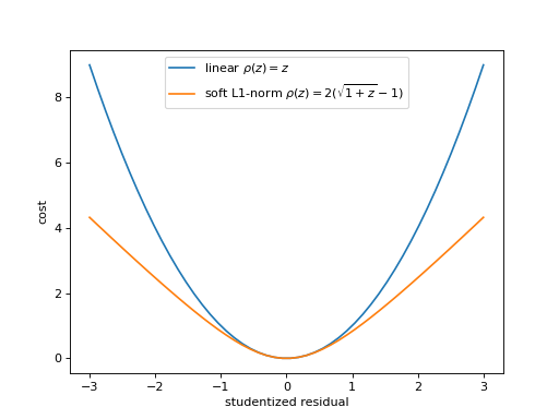
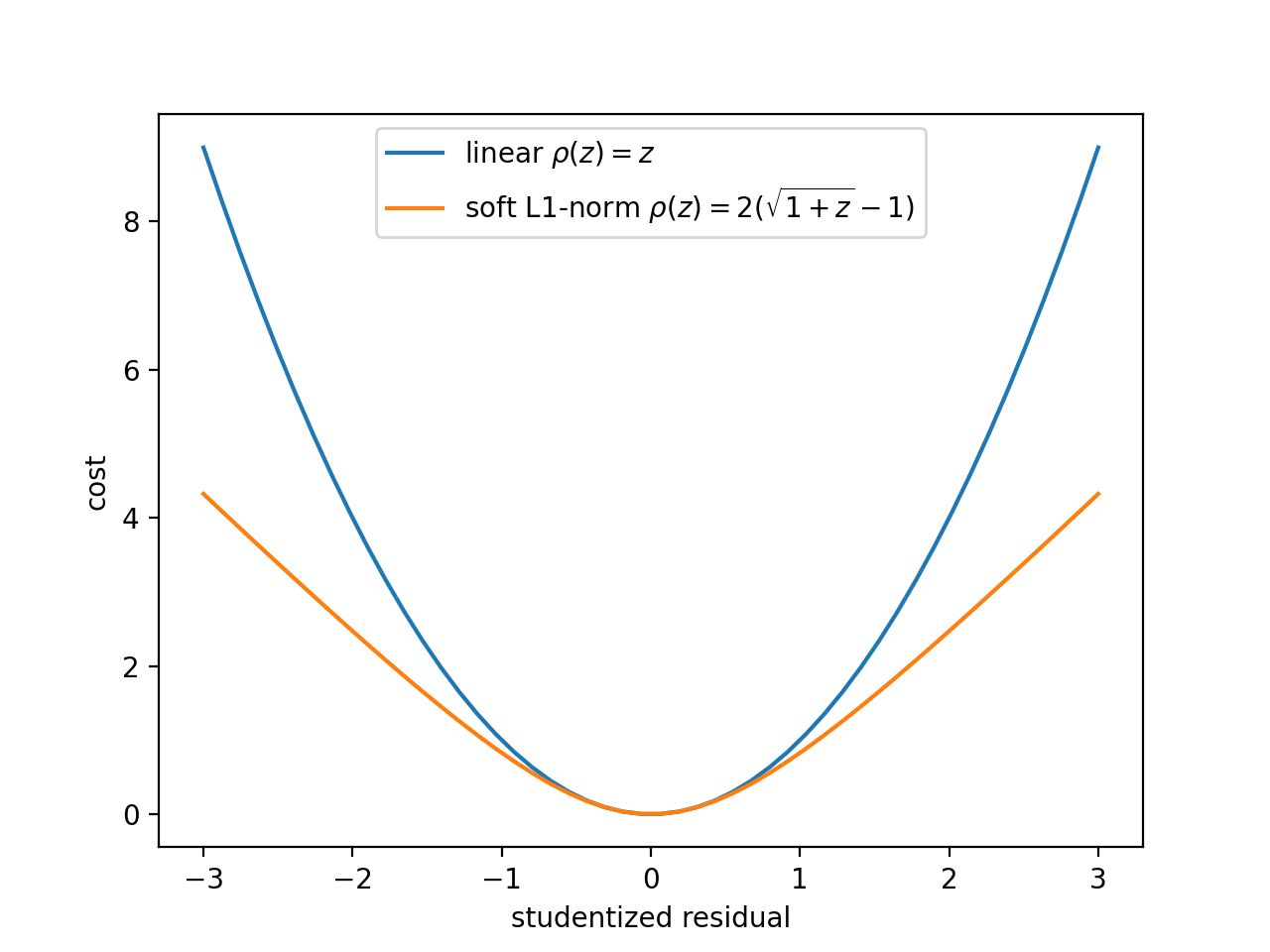
loss (str or callable, optional) – The loss function can be modified to make the fit robust against outliers, see scipy.optimize.least_squares for details. Only “linear” (default) and “soft_l1” are currently implemented, but users can pass any loss function as this argument. It should be a monotonic, twice differentiable function, which accepts the squared residual and returns a modified squared residual.
verbose (int, optional) – Verbosity level. 0: is no output (default). 1: print current args and negative log-likelihood value.

Notes

Alternative loss functions make the fit more robust against outliers by weakening the pull of outliers. The mechanical analog of a least-squares fit is a system with attractive forces. The points pull the model towards them with a force whose potential is given by \(rho(z)\) for a squared-offset \(z\). The plot shows the standard potential in comparison with the weaker soft-l1 potential, in which outliers act with a constant force independent of their distance.

(Source code, png, hires.png, pdf)

prediction(args: Sequence[float]) → ndarray[Any, dtype[ScalarType]]

Return the prediction from the fitted model.

Parameters:: args (array-like) – Parameter values.
Returns:: Model prediction for each bin.
Return type:: NDArray

pulls(args: Sequence[float]) → ndarray[Any, dtype[ScalarType]]

Return studentized residuals (aka pulls).

Parameters:: args (sequence of float) – Parameter values.
Returns:: Array of pull values. If the cost function is masked, the array contains NaN values where the mask value is False.
Return type:: array

Notes

Pulls allow one to estimate how well a model fits the data. A pull is a value computed for each data bin. It is given by (observed - predicted) / standard-deviation. If the model is correct, the expectation value of each pull is zero and its variance is one in the asymptotic limit of infinite samples. Under these conditions, the chi-square statistic is computed from the sum of pulls squared has a known probability distribution if the model is correct. It therefore serves as a goodness-of-fit statistic.

Beware: the sum of pulls squared in general is not identical to the value returned by the cost function, even if the cost function returns a chi-square distributed test-statistic. The cost function is computed in a slightly differently way that makes the return value approach the asymptotic chi-square distribution faster than a test statistic based on sum of pulls squared. In summary, only use pulls for plots. Compute the chi-square test statistic directly from the cost function.

Visualize data and model agreement (requires matplotlib).

The visualization is drawn with matplotlib.pyplot into the current axes.

Parameters:

args (array-like) – Parameter values.
model_points (int or array-like, optional) – How many points to use to draw the model. Default is 0, in this case an smart sampling algorithm selects the number of points. If array-like, it is interpreted as the point locations.

property data: Return data samples.

property loss: Get loss function.

property mask

Boolean array, array of indices, or None.

If not None, only values selected by the mask are considered. The mask acts on the first dimension of a value array, i.e. values[mask]. Default is None.

property model: Get model of the form y = f(x, par0, [par1, …]).

property ndata

Return number of points in least-squares fits or bins in a binned fit.

Infinity is returned if the cost function is unbinned. This is used by Minuit to compute the reduced chi2, a goodness-of-fit estimate.

property verbose

Access verbosity level.

Set this to 1 to print all function calls with input and output.

property x: Get explanatory variables.

property y: Get samples.

property yerror: Get sample uncertainties.

Binned cost function for a template fit with uncertainties on the template.

This cost function is for a mixture of components. Use this if the sample originate from two or more components and you are interested in estimating the yield that originates from one or more components. In high-energy physics, one component is often a peaking signal over a smooth background component. A component can be described by a parametric model or a template.

A parametric model is accepted in form of a scaled cumulative density function, while a template is a non-parametric shape estimate obtained by histogramming a Monte-Carlo simulation. Even if the Monte-Carlo simulation is asymptotically correct, estimating the shape from a finite simulation sample introduces some uncertainty. This cost function takes that additional uncertainty into account.

There are several ways to fit templates and take the sampling uncertainty into account. Barlow and Beeston [1] found an exact likelihood for this problem, with one nuisance parameter per component per bin. Solving this likelihood is somewhat challenging though. The Barlow-Beeston likelihood also does not handle the additional uncertainty in weighted templates unless the weights per bin are all equal.

Other works [2] [3] [4] describe likelihoods that use only one nuisance parameter per bin, which is an approximation. Some marginalize over the nuisance parameters with some prior, while others profile over the nuisance parameter. This class implements several of these methods. The default method is the one which performs best under most conditions, according to current knowledge. The default may change if this assessment changes.

The cost function returns an asymptotically chi-square distributed test statistic, except for the method “asy”, where it is the negative logarithm of the marginalised likelihood instead. The standard transform [5] which we use convert likelihoods into test statistics only works for (profiled) likelihoods, not for likelihoods marginalized over a prior.

All methods implemented here have been generalized to work with both weighted data and weighted templates, under the assumption that the weights are independent of the data. This is not the case for sWeights, and the uncertaintes for results obtained with sWeights will only be approximately correct [6]. The methods have been further generalized to allow fitting a mixture of parametric models and templates.

Initialize cost function with data and model.

Parameters:

n (array-like) – Histogram counts. If this is an array with dimension D+1, where D is the number of histogram axes, then the last dimension must have two elements and is interpreted as pairs of sum of weights and sum of weights squared.
xe (array-like or collection of array-like) – Bin edge locations, must be len(n) + 1, where n is the number of bins. If the histogram has more than one axis, xe must be a collection of the bin edge locations along each axis.
model_or_template (collection of array-like or callable) – Collection of models or arrays. An array represent the histogram counts of a template. The template histograms must use the same axes as the data histogram. If the counts are represented by an array with dimension D+1, where D is the number of histogram axes, then the last dimension must have two elements and is interpreted as pairs of sum of weights and sum of weights squared. Callables must return the model cdf evaluated as xe.
name (collection of str, optional) – Optional name for the yield of each template and the parameter of each model (in order). Must have the same length as there are templates and model parameters in templates_or_model.
verbose (int, optional) – Verbosity level. 0: is no output (default). 1: print current args and negative log-likelihood value.
method ({"jsc", "asy", "da"}, optional) – Which method to use. “jsc”: Conway’s method [2]. “asy”: ASY method [3]. “da”: DA method [4]. Default is “da”, which to current knowledge offers the best overall performance. The default may change in the future, so please set this parameter explicitly in code that has to be stable. For all methods except the “asy” method, the minimum value is chi-square distributed.

prediction(args: Sequence[float]) → Tuple[ndarray[Any, dtype[ScalarType]], ndarray[Any, dtype[ScalarType]]]

Return the fitted template and its standard deviation.

This returns the prediction from the templates, the sum over the products of the template yields with the normalized templates. The standard deviation is returned as the second argument, this is the estimated uncertainty of the fitted template alone. It is obtained via error propagation, taking the statistical uncertainty in the template into account, but regarding the yields as parameters without uncertainty.

Parameters:: args (array-like) – Parameter values.
Returns:: y, yerr – Template prediction and its standard deviation, based on the statistical uncertainty of the template only.
Return type:: NDArray, np.array

pulls(args: Sequence[float]) → ndarray[Any, dtype[ScalarType]]

Return studentized residuals (aka pulls).

Parameters:: args (sequence of float) – Parameter values.
Returns:: Array of pull values. If the cost function is masked, the array contains NaN values where the mask value is False.
Return type:: array

Notes

Pulls allow one to estimate how well a model fits the data. A pull is a value computed for each data bin. It is given by (observed - predicted) / standard-deviation. If the model is correct, the expectation value of each pull is zero and its variance is one in the asymptotic limit of infinite samples. Under these conditions, the chi-square statistic is computed from the sum of pulls squared has a known probability distribution if the model is correct. It therefore serves as a goodness-of-fit statistic.

Beware: the sum of pulls squared in general is not identical to the value returned by the cost function, even if the cost function returns a chi-square distributed test-statistic. The cost function is computed in a slightly differently way that makes the return value approach the asymptotic chi-square distribution faster than a test statistic based on sum of pulls squared. In summary, only use pulls for plots. Compute the chi-square test statistic directly from the cost function.

visualize(args: Sequence[float]) → None

Visualize data and model agreement (requires matplotlib).

The visualization is drawn with matplotlib.pyplot into the current axes.

Parameters:: args (sequence of float) – Parameter values.

Notes

The automatically provided visualization for multi-dimensional data set is often not very pretty, but still helps to judge whether the fit is reasonable. Since there is no obvious way to draw higher dimensional data with error bars in comparison to a model, the visualization shows all data bins as a single sequence.

property data: Return data samples.

property mask

Boolean array, array of indices, or None.

If not None, only values selected by the mask are considered. The mask acts on the first dimension of a value array, i.e. values[mask]. Default is None.

property n: Return data samples.

property ndata

Return number of points in least-squares fits or bins in a binned fit.

Infinity is returned if the cost function is unbinned. This is used by Minuit to compute the reduced chi2, a goodness-of-fit estimate.

property verbose

Access verbosity level.

Set this to 1 to print all function calls with input and output.

property xe: Access bin edges.

Unbinned negative log-likelihood.

Use this if only the shape of the fitted PDF is of interest and the original unbinned data is available. The data can be one- or multi-dimensional.

Initialize UnbinnedNLL with data and model.

Parameters:

data (array-like) – Sample of observations. If the observations are multidimensional, data must have the shape (D, N), where D is the number of dimensions and N the number of data points.
pdf (callable) – Probability density function of the form f(data, par0, [par1, …]), where data is the data sample and par0, … are model parameters. If the data are multivariate, data passed to f has shape (D, N), where D is the number of dimensions and N the number of data points.
verbose (int, optional) – Verbosity level. 0: is no output (default). 1: print current args and negative log-likelihood value.
log (bool, optional) – Distributions of the exponential family (normal, exponential, poisson, …) allow one to compute the logarithm of the pdf directly, which is more accurate and efficient than effectively doing log(exp(logpdf)). Set this to True, if the model returns the logarithm of the pdf instead of the pdf. Default is False.

property data: Return data samples.

property mask

Boolean array, array of indices, or None.

If not None, only values selected by the mask are considered. The mask acts on the first dimension of a value array, i.e. values[mask]. Default is None.

property ndata

Return number of points in least-squares fits or bins in a binned fit.

Infinity is returned if the cost function is unbinned. This is used by Minuit to compute the reduced chi2, a goodness-of-fit estimate.

property pdf: Get probability density model.

property scaled_pdf: Get number density model.

property verbose

Access verbosity level.

Set this to 1 to print all function calls with input and output.

Compute (potentially) chi2-distributed cost.

The value returned by this function is chi2-distributed, if the observed values are normally distributed around the expected values with the provided standard deviations.

Parameters:

y (array-like) – Observed values.
ye (array-like) – Uncertainties of values.
ym (array-like) – Expected values.

Returns:

Const function value.

Return type:

float

Compute asymptotically chi2-distributed cost for binomially-distributed data.

See Baker & Cousins, NIM 221 (1984) 437-442.

Parameters:

n (array-like) – Observed counts.
mu (array-like) – Expected counts per bin. Must satisfy sum(mu) == sum(n).

Returns:

Cost function value.

Return type:

float

Notes

The implementation makes the result asymptotically chi2-distributed and keeps the sum small near the minimum, which helps to maximise the numerical accuracy for Minuit.

Compute asymptotically chi2-distributed cost for Poisson-distributed data.

See Baker & Cousins, NIM 221 (1984) 437-442.

Parameters:

n (array-like) – Observed counts.
mu (array-like) – Expected counts.

Returns:

Cost function value.

Return type:

float

Notes

The implementation makes the result asymptotically chi2-distributed, which helps to maximise the numerical accuracy for Minuit.

Compute asymptotically chi2-distributed cost for a template fit.

H.P. Dembinski, A. Abdelmotteleb, https://doi.org/10.48550/arXiv.2206.12346

Parameters:

n (array-like) – Observed counts.
mu (array-like) – Expected counts. This is the sum of the normalised templates scaled with the component yields.
mu_var (array-like) – Expected variance of mu. Must be positive everywhere.

Returns:

Asymptotically chi-square-distributed test statistic.

Return type:

float

Compute asymptotically chi2-distributed cost for a template fit.

J.S. Conway, PHYSTAT 2011, https://doi.org/10.48550/arXiv.1103.0354

Parameters:

n (array-like) – Observed counts.
mu (array-like) – Expected counts. This is the sum of the normalised templates scaled with the component yields. Must be positive everywhere.
mu_var (array-like) – Expected variance of mu. Must be positive everywhere.

Returns:

Asymptotically chi-square-distributed test statistic.

Return type:

float

Notes

The implementation deviates slightly from the paper by making the result asymptotically chi2-distributed, which helps to maximise the numerical accuracy for Minuit.

Compute marginalized negative log-likelikihood for a template fit.

This is the negative logarithm of equation 3.15 of the paper by C.A. Argüelles, A. Schneider, T. Yuan, https://doi.org/10.1007/JHEP06(2019)030.

The authors use a Bayesian approach and integrate over the nuisance parameters. Like the other Barlow-Beeston-lite methods, this is an approximation. The resulting likelihood cannot be turned into an asymptotically chi-square distributed test statistic as detailed in Baker & Cousins, NIM 221 (1984) 437-442.

Parameters:

n (array-like) – Observed counts.
mu (array-like) – Expected counts. This is the sum of the normalised templates scaled with the component yields.
mu_var (array-like) – Expected variance of mu. Must be positive everywhere.

Returns:

Negative log-likelihood function value.

Return type:

float

Utilities

Data classes and utilities used by iminuit.Minuit.

You can look up the interface of data classes that iminuit uses here.

exception iminuit.util.HesseFailedWarning

HESSE failed warning.

with_traceback(): Exception.with_traceback(tb) – set self.__traceback__ to tb and return self.

exception iminuit.util.IMinuitWarning

Generic iminuit warning.

with_traceback(): Exception.with_traceback(tb) – set self.__traceback__ to tb and return self.

exception iminuit.util.PerformanceWarning

Warning about performance issues.

with_traceback(): Exception.with_traceback(tb) – set self.__traceback__ to tb and return self.

class iminuit.util.FMin(fmin: Any, algorithm: str, nfcn: int, ngrad: int, ndof: int, edm_goal: float, time: float)

Function minimum view.

This object provides detailed metadata about the function minimum. Inspect this to check what exactly happened if the fit did not converge. Use the attribute iminuit.Minuit.fmin to get the best fit values, their uncertainties, or the function value at the minimum. For convenience, you can also get a basic OK from iminuit.Minuit with the methods iminuit.Minuit.valid and iminuit.Minuit.accurate.

property algorithm: str: Get algorithm that was used to compute the function minimum.

property edm: float

Get Estimated Distance to Minimum.

Minuit uses this criterion to determine whether the fit converged. It depends on the gradient and the Hessian matrix. It measures how well the current second order expansion around the function minimum describes the function, by taking the difference between the predicted (based on gradient and Hessian) function value at the minimum and the actual value.

property edm_goal: float

Get EDM threshold value for stopping the minimization.

The threshold is allowed to be violated by a factor of 10 in some situations.

property errordef: float: Equal to the value of iminuit.Minuit.errordef when Migrad ran.

property fval: float: Get cost function value at the minimum.

property has_accurate_covar: bool

Return whether the covariance matrix is accurate.

While Migrad runs, it computes an approximation to the current Hessian matrix. If the strategy is set to 0 or if the fit did not converge, the inverse of this approximation is returned instead of the inverse of the accurately computed Hessian matrix. This property returns False if the approximation has been returned instead of an accurate matrix computed by the Hesse method.

property has_covariance: bool

Return whether a covariance matrix was computed at all.

This is false if the Simplex minimization algorithm was used instead of Migrad, in which no approximation to the Hessian is computed.

property has_made_posdef_covar: bool

Return whether the matrix was forced to be positive definite.

While Migrad runs, it computes an approximation to the current Hessian matrix. It can happen that this approximation is not positive definite, but that is required to compute the next Newton step. Migrad then adds an appropriate diagonal matrix to enforce positive definiteness.

If the fit has converged successfully, this should always return False. If Minuit forced the matrix to be positive definite, the parameter uncertainties are false, see has_posdef_covar for more details.

property has_parameters_at_limit: bool

Return whether any bounded parameter was fitted close to a bound.

The estimated error for the affected parameters is usually off. May be an indication to remove or loosen the limits on the affected parameter.

property has_posdef_covar: bool

Return whether the Hessian matrix is positive definite.

This must be the case if the extremum is a minimum, otherwise it is a saddle point. If it returns False, the fitted result may be correct, but the reported uncertainties are false. This may affect some parameters or all of them. Possible causes:

Model contains redundanted parameters that are 100% correlated. Fix: remove the parameters that are 100% correlated.

Cost function is not computed in double precision. Fix: try adjusting iminuit.Minuit.precision or change the cost function to compute in double precision.
Cost function is not analytical near the minimum. Fix: change the cost function to something analytical. Functions are not analytical if:
It does computations based on (pseudo)random numbers.
It contains vertical steps, for example from code like this:
if cond:
    return value1
else:
    return value2

property has_reached_call_limit: bool

Return whether Migrad exceeded the allowed number of function calls.

Returns True true, the fit was stopped before convergence was reached; otherwise returns False.

property has_valid_parameters: bool

Return whether parameters are valid.

This is the same as is_valid and only kept for backward compatibility.

property hesse_failed: bool: Return whether the last call to Hesse failed.

property is_above_max_edm: bool

Return whether the EDM value is below the convergence threshold.

Returns True, if the fit did not converge; otherwise returns False.

property is_valid: bool

Return whether Migrad converged successfully.

For it to return True, the following conditions need to be fulfilled:

has_reached_call_limit is False

is_above_max_edm is False

Note: The actual verdict is computed inside the Minuit2 C++ code, so we cannot guarantee that is_valid is exactly equivalent to these conditions.

property nfcn: int: Get number of function calls so far.

property ngrad: int: Get number of function gradient calls so far.

property reduced_chi2: float

Get χ²/ndof of the fit.

This returns NaN if the cost function is unbinned, errordef is not 1, or if the cost function does not report the degrees of freedom.

property time: float: Runtime of the last algorithm.

class iminuit.util.FixedView(minuit: Any, ndim: int = 0)

Array-like view of whether parameters are fixed.

to_dict() → Dict[str, float]: Obtain dict representation.

class iminuit.util.LimitView(minuit: Any)

Array-like view of parameter limits.

to_dict() → Dict[str, float]: Obtain dict representation.

class iminuit.util.MError(*args: int | str | float | bool)

Minos data object.

number

Parameter index.

Type:: int

name

Parameter name.

Type:: str

lower

Lower error.

Type:: float

upper

Upper error.

Type:: float

is_valid

Whether Minos computation was successful.

Type:: bool

lower_valid

Whether downward scan was successful.

Type:: bool

upper_valid

Whether upward scan was successful.

Type:: bool

at_lower_limit

Whether scan reached lower limit.

Type:: bool

at_upper_limit

Whether scan reached upper limit.

Type:: bool

at_lower_max_fcn

Whether allowed number of function evaluations was exhausted.

Type:: bool

at_upper_max_fcn

Whether allowed number of function evaluations was exhausted.

Type:: bool

lower_new_min

Parameter value for new minimum, if one was found in downward scan.

Type:: float

upper_new_min

Parameter value for new minimum, if one was found in upward scan.

Type:: float

nfcn

Number of function calls.

Type:: int

min

Function value at the new minimum.

Type:: float

class iminuit.util.MErrors

Dict-like map from parameter name to Minos result object.

clear() → None. Remove all items from od.

copy() → a shallow copy of od

fromkeys(value=None): Create a new ordered dictionary with keys from iterable and values set to value.

get(key, default=None, /): Return the value for key if key is in the dictionary, else default.

items() → a set-like object providing a view on D's items

keys() → a set-like object providing a view on D's keys

move_to_end(key, last=True)

Move an existing element to the end (or beginning if last is false).

Raise KeyError if the element does not exist.

pop(key[, default]) → v, remove specified key and return the corresponding value.: If the key is not found, return the default if given; otherwise, raise a KeyError.

popitem(last=True)

Remove and return a (key, value) pair from the dictionary.

Pairs are returned in LIFO order if last is true or FIFO order if false.

setdefault(key, default=None)

Insert key with a value of default if key is not in the dictionary.

Return the value for key if key is in the dictionary, else default.

update([E, ]**F) → None. Update D from dict/iterable E and F.: If E is present and has a .keys() method, then does: for k in E: D[k] = E[k] If E is present and lacks a .keys() method, then does: for k, v in E: D[k] = v In either case, this is followed by: for k in F: D[k] = F[k]

values() → an object providing a view on D's values

Data object for a single Parameter.

property has_limits: Query whether the parameter has an lower or upper limit.

property has_lower_limit: Query whether parameter has a lower limit.

property has_upper_limit: Query whether parameter has an upper limit.

class iminuit.util.Params(iterable=(), /)

Tuple-like holder of parameter data objects.

count(value, /): Return number of occurrences of value.

index(value, start=0, stop=9223372036854775807, /)

Return first index of value.

Raises ValueError if the value is not present.

to_table()

Convert parameter data to a tabular format.

The output is consumable by the external tabulate module.

Examples

>>> import tabulate as tab
>>> from iminuit import Minuit
>>> m = Minuit(lambda x, y: x ** 2 + (y / 2) ** 2 + 1, x=0, y=0)
>>> m.fixed["x"] = True
>>> m.migrad().minos()
>>> tab.tabulate(*m.params.to_table())
  pos  name      value    error  error-    error+    limit-    limit+    fixed
-----  ------  -------  -------  --------  --------  --------  --------  -------
    0  x             0      0.1                                          yes
    1  y             0      1.4  -1.0      1.0

class iminuit.util.ValueView(minuit: Any, ndim: int = 0)

Array-like view of parameter values.

to_dict() → Dict[str, float]: Obtain dict representation.

iminuit.util.describe(callable: Callable) → List[str]

iminuit.util.describe(callable: Callable, annotations: bool) → Dict[str, Tuple[float, float] | None]

Attempt to extract the function argument names and annotations.

Parameters:

callable (callable) – Callable whose parameters should be extracted.
annotations (bool, optional) – Whether to also extract annotations. Default is false.

Returns:

If annotate is False, return list of strings with the parameters names if successful and an empty list otherwise. If annotations is True, return a dict, which maps parameter names to annotations. For parameters without annotations, the dict maps to None.

Return type:

list or dict

Notes

Parameter names are extracted with the following three methods, which are attempted in order. The first to succeed determines the result.

Using obj._parameters, which is a dict that makes parameter names to parameter limits or None if the parameter has to limits. Users are encouraged to use this mechanism to provide signatures for objects that otherwise would not have a detectable signature. Example:
```
def f(*args):  # no signature
    x, y = args
    return (x - 2) ** 2 + (y - 3) ** 2

f._parameters = {"x": None, "y": (1, 4)}
```
Here, the first parameter is declared to have no limits (values from minus to plus infinity are allowed), while the second parameter is declared to have limits, it cannot be smaller than 1 or larger than 4.

Note: In the past, the func_code attribute was used for a similar purpose as _parameters. It is still supported for legacy code, but should not be used anymore in new code, since it does not support declaring parameter limits.

If an objects has a func_code attribute, it is used to detect the parameters. Example:
```
from iminuit.util import make_func_code

def f(*args): # no signature
    x, y = args
    return (x - 2) ** 2 + (y - 3) ** 2

# deprecated, make_func_code will raise a warning
f.func_code = make_func_code(("x", "y"))
```
Using inspect.signature(). The inspect module provides a general function to extract the signature of a Python callable. It works on most callables, including Functors like this:
```
class MyLeastSquares:
    def __call__(self, a, b):
        ...
```
Limits are supported via annotations, using the Annotated type that was introduced in Python-3.9 and can be obtained from the external package typing_extensions in Python-3.8. In the following example, the second parameter has a lower limit at 0, because it must be positive:
```
from typing import Annotated

def my_cost_function(a: float, b: Annotated[float, 0:]):
    ...
```
There are no standard annotations yet at the time of this writing. iminuit supports the annotations Gt, Ge, Lt, Le from the external package annotated-types, and interprets slice notation as limits.
Using the docstring. The docstring is textually parsed to detect the parameter names. This requires that a docstring is present which follows the Python standard formatting for function signatures.

Ambiguous cases with positional and keyword argument are handled in the following way:

# describe returns [a, b];
# *args and **kwargs are ignored
def fcn(a, b, *args, **kwargs): ...

# describe returns [a, b, c];
# positional arguments with default values are detected
def fcn(a, b, c=1): ...

iminuit.util.make_func_code(*args, **kwargs): deprecated: Use of func_code attribute to declare parameters is deprecated. Use _parameters instead, which is a dict of parameter names to limits.

iminuit.util.make_with_signature(callable: Callable, *varnames: str, **replacements: str) → Callable

Return new callable with altered signature.

Parameters:

callable – Original callable whose signature shall be changed.
*varnames (sequence of str) – Replace the first N argument names with these.
**replacements (mapping of str to str, optional) – Replace old argument name (key) with new argument name (value).

Return type:

callable with new argument names.

iminuit.util.merge_signatures(callables: Iterable[Callable], annotations: bool = False) → Tuple[Any, List[Tuple[int, ...]]]

Merge signatures of callables with positional arguments.

This is best explained by an example:

def f(x, y, z): ...

def g(x, p): ...

parameters, mapping = merge_signatures(f, g)
# parameters is ('x', 'y', 'z', 'p')
# mapping is ((0, 1, 2), (0, 3))

Parameters:

callables – Callables whose parameters can be extracted with describe().
annotations (bool, optional) – Whether to return the annotions. Default is False, for backward compatibility.

Returns:

parameters is the tuple of the merged parameter names. mapping contains the mapping of parameters indices from the merged signature to the original signatures.

Return type:

tuple(parameters, mapping)

class iminuit.util.Matrix(parameters: Dict | Tuple)

Enhanced Numpy ndarray.

Works like a normal ndarray in computations, but also supports pretty printing in ipython and Jupyter notebooks. Elements can be accessed via indices or parameter names.

correlation()

Compute and return correlation matrix.

If the matrix is already a correlation matrix, this effectively returns a copy of the original matrix.

to_dict() → Dict[Tuple[str, str], float]

Convert matrix to dict.

Since the matrix is symmetric, the dict only contains the upper triangular matrix.

to_table() → Tuple[List[List[str]], Tuple[str, ...]]

Convert matrix to tabular format.

The output is consumable by the external tabulate module.

Examples

>>> import tabulate as tab
>>> from iminuit import Minuit
>>> m = Minuit(lambda x, y: x ** 2 + y ** 2, x=1, y=2).migrad()
>>> tab.tabulate(*m.covariance.to_table())
      x    y
--  ---  ---
x     1   -0
y    -0    4